ABSTRACT
The data covering Mayo Daga and Gashaka areas of Taraba State has been interpreted by applying source parameter imaging (SPI) and forward and inverse modeling methods. From the quantitative method of interpretation, it was found out that the magnetic intensity within the study area ranges from -129.9 to 186.6 nT in which the area is noticeably marked by both low and high magnetic signatures which may be as a result of several factors such as; susceptibility, degree of strike, difference in magnetic variation in depth and difference in lithology. From the quantitative interpretation, depth estimates obtained when SPI is employed shown minimum to maximum depth to anomalous source that ranges from 400.7 to 2119.2 m. Forward and inverse modeling estimated depths for profiles P1, P2, P3, and P4 were 2372, 2537, 1621 and 1586 m, respectively, with susceptibility values of 0.0754, 0.0251, 0.0028, and 0.001 respectively, suggesting that the bodies causing the anomaly are typical of igneous rocks; basalt and olivine, intermediate igneous rock; granites, and rocks mineral (quartz).
Key words: Aeromagnetic data, source parameter imaging (SPI), qualitative and quantitative interpretation
Minerals and hydrocarbon play vital roles in the socio-economic development of a country of which Nigeria is not an exception. Aeromagnetic surveys are widely used to aid production of geological maps, regional geological studies, location and definition of buried metallic objects, engineering site investigation, archeo-geophysics and are also commonly used for mineral exploration by detecting minerals or rocks with unusual magnetic properties which reveal themselves by causing anomalies in the magnetic field intensity of the earth. Aeromagnetic maps usually show changes in the earth’s magnetic field resulting from the properties of rock sediments (e.g. magnetic susceptibilities). Basic igneous rocks have the highest magnetic susceptibility, while acidic igneous rocks have intermediate magnetic susceptibility and sedimentary rocks have the lowest magnetic (Kearey et al., 2002). Some minerals deposits are associated with abundance of magnetic minerals, and occasionally the target may itself be magnetic (e.g. iron ore deposits), but often the elucidation of surface structure of the upper crust is the most valuable contribution of the aeromagnetic data (Hamza and Garba, 2010). This method plays a distinguished role when compared with other geophysical methods, it is cheaper, faster and large area of land especially areas of political barrier, economic, social and environmentally hazardous can easily be covered. The main purpose of this work is to study the magnetic anomalies of Mayo Daga and Gashaka areas, by interpreting qualitatively and quantitatively the aeromagnetic anomaly of the areas. The purposes are; to estimate the basement depth, to determine the magnetic susceptibility and type of mineralization prevalent in the area.
Location and geology of the study area
The study area is located in Mambilla Plateau, Sardauna Local Government Area of Taraba State. It is located between latitude 5°30' to 7°18' and longitude 10°18' to 11°37' having a total land mass of 3,765.2 km2 and forms the southernmost tip of east of northern part of Nigeria (Tukur et al., 2005). This plateau is Cameroon-locked in the southern, eastern and western part as shown in Figure 1 (Frantz, 1981). According to Mubi and Tukur (2005), the basement complex rocks underlay more than two-third of the plateau and dates back to the Precambrian to early Paleozoic era. Meanwhile, according to Jeje (1983), the remaining part of the plateau is made up of volcanic rocks of the upper Cenozoic to tertiary and quaternary ages. These rocks found within the plateau are of volcanic origin, extended from tectonic lines, fissures, etc. These volcanic rocks comprises olivine basalt, basalts suite and trachyte basalt which were found to contain mixtures of amphiboles, pyroxenes with some other free minerals of quartz (Mould, 1960). The tertiary basalts are found in the Mambilla Plateau mostly formed by trachytic lavas and extensive basalts (Dupreez and Barber, 1995).

DATA SOURCE AND METHODOLOGY
The data covering the study area was obtained from Nigeria Geological Survey Agency (NGSA). The company, FURGRO Airborne Surveys in collaboration with Federal Government of Nigeria and World Bank carried out the acquisition and processing of data with a terrain clearance of 100 m, altitude of 80 m, 100 m flight line spacing and 500 m tie line spacing. The data obtained from NGSA is in digitized form, XYZ format. The first stage of interpretation is gridding; it is a process of interpolating data unto an equally spaced grid of cells in a specified coordinate system. Because the XYZ data were collected over widely separated parallel lines which may have resulted in some points along the survey not sampled, it is important that we represent the sampled data by determining the values at points equally spaced far apart at the nodes of a grid. To produce the grids, “minimum curvature” method was used (Briggs, 1974). This method, also called the random gridding method, fit a minimum curvature surface to data points. The method was used because the data were sparely sampled over wide area and continuous between data points. The RANGRID GX of the Oasis Montaj software was used to achieve this. Here, a grid size of 300 m was used to avoid over or under sampling based on the sampling distance of the data.
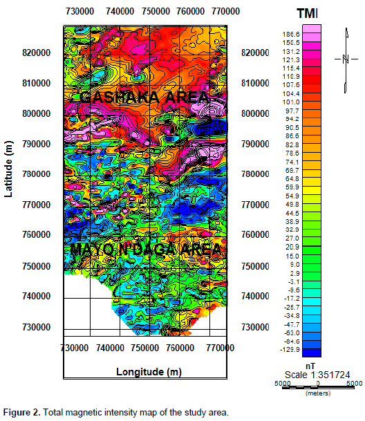
The quantitative interpretation of the aeromagnetic data of the study area was carried out by inspecting the TMI gridded map. This map is in colour aggregate, and the general purpose is to gain some preliminary information of source of anomalies (Obiora et al., 2016). Oasis Montaj software was employed in producing the total intensity (TMI) map. From the map, one can talk of certain features about the magnetic intensity and the factors (such as susceptibility, depth to the magnetic bodies, nature of the bodies, etc) responsible for the change in magnetic signatures. The regional anomaly was separated from the residual anomaly by applying first order polynomial which was fitted by least square method to the data. Different orders of polynomial were tried and it was found that the first order polynomial fitting was the best for our data as it reflected the geological information of the area. The equation used to generate the algorithm for removal of regional data according to Ugwu et al. (2013) is given as:

where

is the regional field,

are the X and Y coordinates of the geographical centre of the dataset respectively. And

are the regional polynomial coefficients.
Quantitative interpretation of aeromagnetic data involves making numerical estimates of dimensions and depth of the anomalies and often takes the form of sources’ modelling theoretically replicating the recorded anomalies during the survey. In order to see whether the earth model is consistent with what has been observed, that is, developing a model that is suitable in terms of physical approximation to the unknown geology, conceptual models of the subsurface are created and its anomalies calculated. Quantitatively, forward and inverse modelling and source parameter imaging (SPI) was employed in this research work. Forward modelling involves comparing of the calculated field with observed data, in which the models are adjusted to improve the fitting of the calculated and observed data. In comparing the calculated field of a hypothetical source with that of the observed data, the model is adjusted in order to improve the fit for a subsequent comparison. This technique makes use of trial and error approach to estimate the distribution of magnetization within the source or geometry of the source.
The model may be two- or three- dimensional. In inverse modelling method, some source parameters are determined directly from the measured data which is an opposition to the trial and error or indirect determination. It is customary in this method to constrain some parameters of the source in the way, keeping in mind that every anomaly has an infinite number of permissible sources bringing about infinite number of solutions (Obiora et al., 2016). The inversion of magnetic data may involve one of the following three approaches; Calculation of depth to source or depth to bottom of source, calculation of magnetic distribution given the geometry of the source and calculation of source geometry given the distribution of magnetization. Oasis Montaj containing the Potent software was used in the modelling and inversion of the anomalies in this research work. Potent software is a program used for the modelling of the gravitational and magnetic effects of surface and is well suited for modelling ore body in detail for mineral exploration and providing a highly 3-D interactive environment among other applications. In Potent, the main concept includes; calculation, observation, inversion, model and visualisation and the model consist of an assemblage of simple geometrical bodies. Using Potent, the following geometrical bodies can be created; sphere, rectangular prism, cylinder, dyke, lens, slab, ellipsoid and polygonal prism. By trial and error approach, these bodies were attempted in modelling the observed data in order to obtain the best fit model.
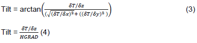
The observed data were best modelled by sphere, dyke, slab and rectangular prism. In trying to model the observed data of the study area, Potent assigns the body default parameters (physical properties, shapes, position). The body created is modelled by varying any of the parameters of the body. In interpreting the observed data, the first step was to take profiles on the field image. In view of this, seven profiles (P1, P2, P3, P4, P5, P6 and P7) were taken at different parts of the field image. The second quantitative method employed was SPI. Estimation of source parameters can be performed on gridded aeromagnetic data. This has two advantages; 1) it eliminates errors caused by the lines of survey that are not perpendicularly oriented to the strike and secondly, it has no dependency on an operator size or user selected window other techniques like Euler methods and Naudy (1970) requires. Furthermore, output quantities grids can be generated and subsequently, image can be processed to enhance detail of structural information that otherwise may not be evident (Abbas and Mallam, 2013). This SPI method utilizes the relationship between the local wave number (k) and the source depth of the observed field, for which calculation of any point within a grid of data through vertical and horizontal gradients can be carried out (Thurston and Smith, 1997). According to Thurston and Smith (1997), the original SPI works only for two models: a sloping contact and a dipping thin dike. The maxima of the local wave number (k) is located above isolated contacts and estimate of depths can be made without assumptions about the thickness of the source of bodies. Using SPI method, grids solutions show the edge location, susceptibility contrast, dips and depths. This method requires first and second order derivatives thus making it susceptible to both interference effects and noise in the data (Abbas and Mallam, 2013). The basics of this method, is that for vertical contacts, the peaks of the k defines the inverse of the depth. Given as;


HGRAD =horizontal gradient, T = total magnetic intensity (TMI).
The SPI method helps in calculating the parameters of source from gridded magnetic data. This method assumes either a 2D dipping thin-sheet model or a 2D slopping contact that is based on the complex analytical signal. The solution grids show the dips, depth, susceptibility contrast and the edge location. The depth estimate is not dependent on magnetic declination, inclination, dip, strike or any remanent magnetization. Processing of the SPI image grids provides and enhances maps that facilitate interpretation by non-specialists (Ojoh, 1992).
RESULTS PRESENTATION AND DISCUSSION
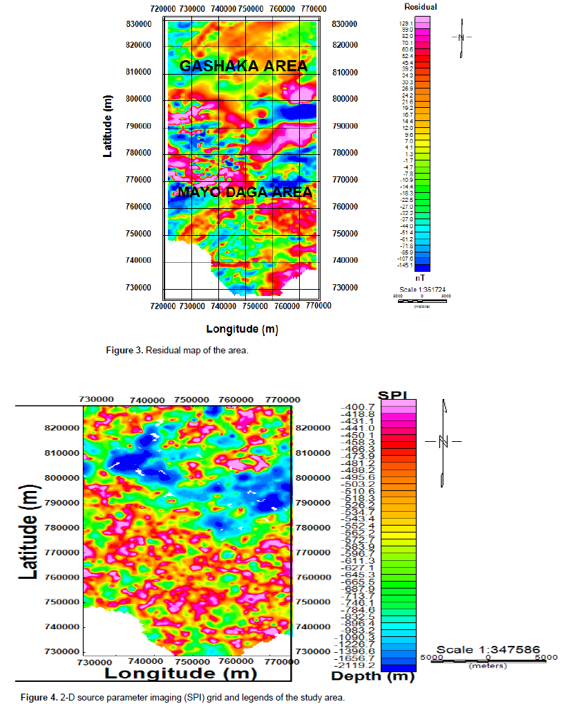
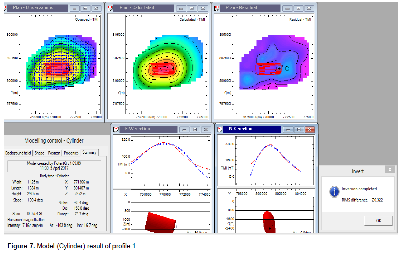
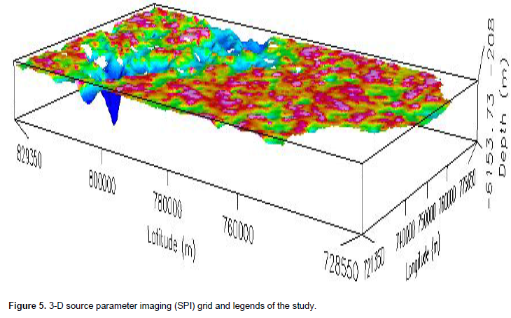
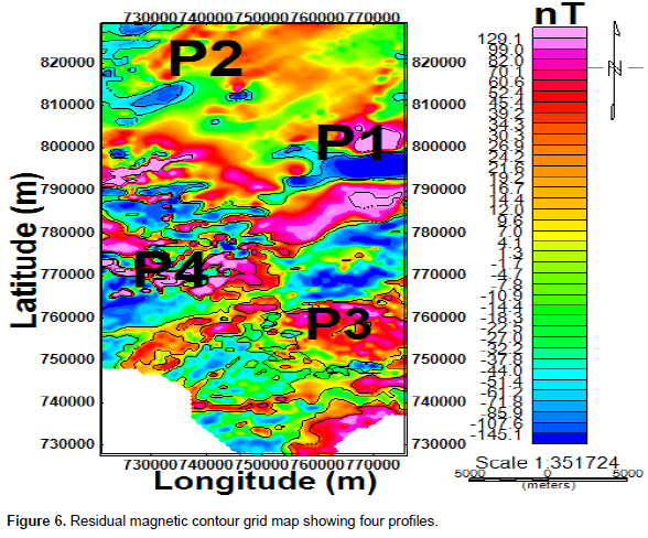
Interpreting the data quantitatively, the data was gridded to produce the total magnetic intensity (TMI) map of the study area which is in colour aggregate (Figure 2). From the TMI map, the magnetic intensity varies between a minimum value of -129.9 nT to a maximum value of 186.6 nT and is marked by both high and low magnetic signatures. These variations may be due to several factors such as; difference in lithology, magnetic susceptibility, variation in degree of strike, depth and difference in lithology. In the northern and southern part of the study area, orientation of the contours is closely spaced. This suggests that local fracture zones or faults may possibly pass via these areas. The elliptically closed contours in the study area equally suggests the presence of magnetic bodies. Most of the anomalous features are trending in the East-western direction. The regional map was separated from the TMI grid to obtain the residual as shown in Figure 3, and ranges from -145.1 to 129.1 with variations in colour as indicated on the legend bar. In computing the SPI depth, Oasis Montaj software and the generated SPI grid image and legend are employed. Figure 4 shows different colours which is an indication of varying magnetic susceptibility contrast within the study area and could equally portray the basement surface undulations. Oasis Montaj software was used in computing the SPI image and depth.


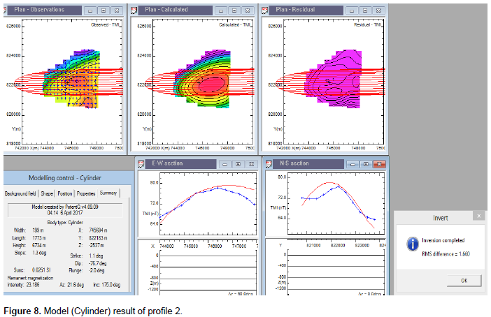
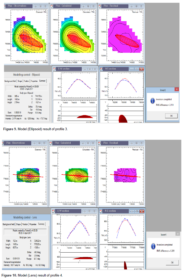
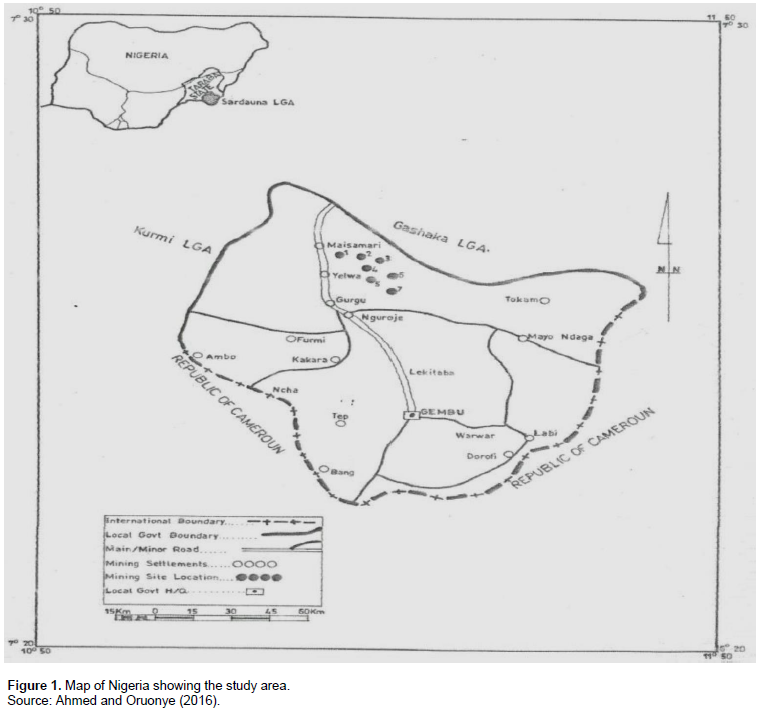
The shape, physical properties and position were adjusted during the forward modelling session in order to obtain a good correlation between the observed and calculated field. Potent was used to calculate the field at the actual observation points (the points where the observed field is known). The field from the model was automatically calculated in response to the changes made to the model. The observed values are shown as an image and as a single E-W and N-S profile. Their fit is measured by their visible superposition and the root mean square (RMS) values. The root mean square (RMS) difference between the calculated and observed values was minimized by the inversion algorithm. At the end of each inversion exercise, the RMS value was displayed. The RMS value of less than twenty-one (21) was set as a standard for the inversion result as the fit between the observed and calculated field; thereafter, the RMS value was displayed at the end of each inversion exercise. As the fit between observed and calculated field continues to improve, the value of RMS continue decreasing until a reasonable inversion result was achieved.
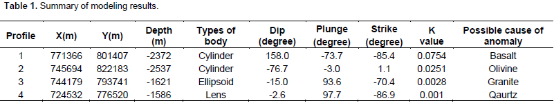
The sub profiles in each model show the variations of the field values with distance at the area or points modelled. Profiles P1 and P2 taken around north-western and north-eastern parts of the study area were modeled by cylinder shapes emplaced at depths of 2372 and 2537 m respectively (Figures 8 and 9). The bodies have magnetic susceptibilities of 0.0754 and 0.0251 respectively suggesting that the bodies causing the anomaly are typical of igneous rocks; basalt and olivine (Telford et al., 1990). Profile P3 taken in the south eastern part was modeled by Ellipsoid shape emplaced at depth of 1621 m with susceptibility value of 0.0028 (Figure 10), suggesting that the bodies causing the anomaly are typical of intermediate igneous rock; granites (Telford et al., 1990). The Profile P4 taken in the south western part of the study area was modeled with Lens shape emplaced at depth of 1586 m with magnetic susceptibility value of 0.001 (Figure 11), revealing rocks mineral (quartz) (Telford et al., 1990). The blue colour in the modeling map (Figure 7) cannot be modeled. The reason could be as a result of very low total magnetic intensity in the area. Table 1 shows the summary of the modelling result.


The magnetic anomalies of Gashaka and Mayo Daga areas were studied by employing qualitative and quantitative interpretation of aeromagnetic data of the area. SPI and forward and inverse modeling methods were used as part of quantitative interpretation. From the interpretation method used, the maximum depths obtained from each method were similar and are approximately 2.3 km each. These three depths obtained from SPI, Euler as well as forward and inverse modeling, are good for hydrocarbon accumulation in the study area, and agrees with the assertion of Wright et al. (1985) that the minimum thickness of the sediment required for the commencement of oil formation from marine organic remains would be 2300 m (2.3 km), if other factors are satisfactory. Through the results from the qualitative and quantitative interpretation obtained from this study, this work has shown some similarities in agreement with those of other researchers (Chinwuko et al., 2013; Wright et al., 1985). However, this present work could be more reliable in terms of terrain clearance, line spacing and improvement in technology. The aeromagnetic study of the area has helped to delineate the geological structures of Gashaka and Mayo Daga areas which are of great benefits to the solid mineral sector of Nigeria economy.
The authors have not declared any conflict of interests.
REFERENCES
|
Abbas AA, Mallam A (2013). Estimating the Thickness of Sedimentation within Lower Benue Basin and Upper Anambra Basin, Nigeria, Using Both Spectral Depth Determination and Source Parameter Imaging. Hindawi Publishing Corporation P 10.
|
|
|
|
Ahmed YM, Oruonye ED (2016). Socioeconomic Impact of Artisanal and Small scale mining on the Mambilla Plateau of Taraba State, Nigeria. World J. Soc. Sci. Res. 3(1).
|
|
|
|
Briggs IC (1974). Machine contouring using minimum curvature. Geophysics 39:39-48.
Crossref
|
|
|
|
Chinwuko AI, Onwuemesi AG, Anakwuba EK, Okeke HC, Onuba LN, Okonkwo CC, Ikumbur EB (2013). Spectral Analysis and Magnetic Modeling over Biu – Damboa, Northeastern Nigeria. IOSR J. Appl. Geol. Geophys. 1(1):20-28.
Crossref
|
|
|
|
Dupreez JW, Barber W (1965). The distribution and chemical quality of ground water in Northern Nigeria. Bulletin 36. Geological survey of Nigeria 93.
|
|
|
|
Frantz C (1981). Development without communities: Social fields, Network and Action in the Mambilla Grasslands of Nigeria. J. Human org. pp. 211-220.
Crossref
|
|
|
|
Hamza H, Graba I (2010). Challenges of exploration and utilization of hydrocarbons in the Sokoto Basin. Paper presented at International Conference on the Potentials of Prospecting for Hydrocarbons in the Sokoto Basin on 11th May, 2009 at Usmanu Danfodio University Sokoto, Nigeria.
|
|
|
|
Jeje LK (1983). Aspects of geomorphology of Nigeria. Heinemann educational books.
|
|
|
|
Kearey P, Brooks M, Hill I (2002). An Introduction to Geophysical Exploration. (3rd edition). Blackwell Publishing. United Kingdom.
|
|
|
|
Mould AWS (1960). Report on a rapid reconnaissance soil survey of the Mambilla plateau. Bulletin 15, Soil survey section, regional research station, ministry of agriculture, Samaru, Zaria.
|
|
|
|
Mubi AM, Tukur AL (2005). Geology and relief of Nigeria. Nigeria. Heinemann educational books.
|
|
|
|
Naudy H (1970). Method for analyzing aeromagnetic profiles. Geophys. Prospect. 18(1):56-63.
Crossref
|
|
|
|
Obiora DN, Yakubu JA, Okeke FN, Chukudebelu JU, Oha AI (2016). Interpretation of Aeromagnetic Data of Idah Area in North Central Nigeria Using Combined Methods. J. Geol. Soc. India 88:98-106.
Crossref
|
|
|
|
Ojoh KA (1992). The southern part of the Benue trough (Nigeria) Cretaceous stratigraphy, basin analysis, paleo-oceanography and geodynamic evolution in the equatorial domain of the south Atlantic. NAPE Bull. 7:131-152.
|
|
|
|
Telford WM, Geldart LP, Sheriff RE (1990). Applied geophysics (2nd edition), Cambridge University press, Cambridge.
Crossref
|
|
|
|
Thurston JB, Smith RS (1997). Automatic conversion of magnetic data to depth, dip, and susceptibility contrast using the SPITM method. Geophysics 62(3):807-813.
Crossref
|
|
|
|
Tukur AL, Adebayo AA, Galtima A (2005). The land and people of the Mambilla Plateau, Nigeria. Heinemann educational books.
|
|
|
|
Ugwu GZ, Ezema PO, Eze CC (2013). Interpretation of aeromagnetic data over Okigwe and Afikpo areas of Lower Benue Trough, Nigeria. Int. Res. J. Geol. Mining 3(1):1-8.
|
|
|
|
Wright JB, Hastings D, Jones WB, Williams HR (1985). Geology and Mineral resources of West Africa. George Allen and Urwin, London.
|


 is the regional field,
  are the X and Y coordinates of the geographical centre of the dataset respectively. And
  are the regional polynomial coefficients.