ABSTRACT
The US labeled China a Currency Manipulator in August 2019 because of the massive trade balance surplus of China. The correlation between RMB’s exchange rate and China’s trade balance has been discussed worldwide. The Traditional Marshal-Lerner Condition states if the sum of the absolute value of export and import price elasticity of demand is more than 1, the trade balance will be adjusted through the fluctuation of the exchange rate. However, Traditional Marshal-Lerner Condition requires trade balance is 0 at the beginning, while China benefits the huge surplus of the trade balance for decades. Therefore, the Traditional Marshal-Lerner Condition may not be appropriate to explain why RMB’s exchange rate failed to shrink the surplus of China’s trade balance. The author reconsiders the derivation of Marshall-Lerner condition and presents another Marshall-Lerner condition which illustrates the conditions the export and import price elasticity of demand need to meet when the trade balance is uneven at the beginning so that the fluctuation of exchange rate can play a role in regulating trade balance. Then the industry-level data from January 2008 to June 2018 were used to calculate the export and import price elasticities of demand by using ARDL model. The empirical results show the validity of Traditional Marshal-Lerner Condition in China was investigated, while the Generalized Marshal-Lerner Condition cannot be satisfied during the sample period. Taking the huge amount of surplus, and the movements of RMB’s exchange rate recent years into consideration, the results of Generalized Marshal-Lerner Condition, that the variation of RMB’s exchange rate will not succeed in adjusting the trade balance in the Chinese economy, maybe more persuasive than the traditional one.
Key words: China, Marshall-Lerner condition, trade balance, ARDL model.
Since China joined the WTO in 2001, China’s economic international standing has been rising rapidly due to the development of international trade. China’s export share, which occupied 6% of the World’s share in 2001, has expanded to around 16% in 2018 significantly, taking the top position in the world. Concerning China’s import share, it has expanded steadily from 5% in 2001 to 13% in 2018, making it the third-largest in the world. That is to say while ensuring its status as a “World’s Factory”, China has also made itself to be a “Global Consumer Market”.
Along with the expansion of China’s trade balance, trade friction between China and other countries is becoming fiercer nowadays. The US implemented treat restrictions such as imposing tariffs on “Made in China” in September 2018. There is a growing debate on the situation of China; now is identical to Japan in the 1990s, the focus of the friction between the US and China is likely to shift from “Trade” to “Exchange Rate”. Since the friction between the US and China started, the tendency for the depreciation of the RMB to the USD rate is accelerated. The US hopes to force China to adjust the RMB’s exchange rate to reach its goal, which is to reverse the situation of the trade imbalance between these two countries. Revaluation of RMB’s exchange rate has been perceived as an effective way to settle the trade disputes between the US and China, and also the driving global imbalances. Since the RMB exchange rate reform in 21st July 2005, which People’s Bank of China (PBC) announced to implement a reform of the exchange rate regime-switching from the ‘Dollar-peg Regime’ to ‘A Managed Floating Regime with Reference to a Currency Basket and the Supply-demand Conditions’, the nominal exchange rate of RMB to USD appreciated to about 17.32%, and the Nominal Effective Exchange Rate (NEER) and Real Effective Exchange Rate (REER) rose by 42.28 and 32.78% respectively. Despite the variation of RMB, China’s trade balance is still having a huge surplus these years. Before the 2008 Financial Crisis, the surplus of China has reached 296.5 billion dollars, and after that, it reached its peak of 601.6 billion dollars in 2015. Therefore, the movements of RMB’s exchange rate failed to adjust the trade balance surplus of China.
The liaison between the exchange rate and trade balance is an imperative basis for the foreign policy of every country. For them, it is a major concern whether the domestic currency’s appreciation or depreciation will have corresponding effects on the trade balance or not. Traditionally, because the appreciation of domestic currency will make the price of export to increase, foreign consumers tend to choose other country’s goods instead. So many economists and politicians believe that the appreciation of domestic currency will decrease the international competitiveness of domestic goods when exporting them to market abroad. While the appreciation of domestic currency will increase domestic consumer’s purchasing power, they will buy more import goods when the domestic currency is appreciated. Hence, the appreciation of domestic currency will lessen export and add import at the same time; it will reduce the trade balance of a country. This opinion is considered as a policymaking instruction to exacerbate the surplus of the trade balance.
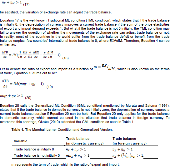
According to the traditional economic theory, the affiliation of the exchange rate and trade balance can to a great extent be explained by the Marshall-Lerner condition (ML Condition) and Pass-through theory. ML condition states that if the sum of price elasticity of demand for export (the extent to export flows) is responsive to relative prices change and price elasticity of demand for import (the extent to import flows is responsive to relative price change) is greater than 1, then the Balance of Trade will be adjusted through the variation of exchange rate. However, this ML Condition is based on many strict assumptions such as the trade balance is initially 0. On the one hand, if a country’s trade balance is even, there is no need to improve the trade balance by alternating the domestic currency’s exchange rate. When a country’s trade balance is uneven, it is necessary to take actions to adjust the imbalance of trade. On the other hand, in reality, most countries suffer from the deficit of trade balance or enjoy the surplus of the trade balance, especially China, which has the largest surplus of trade balance in the world. Therefore, it might not be appropriate to use the ML Condition to discuss whether the movement of RMB’s exchange rate can have an effect on China’s trade balance or not. There are numerous studies about whether China’s export and import price elasticity of demand meets the ML condition or not, but they did not take a full consideration about China’s trade balance is bigger than 0, which is against one assumption of the ML Condition. The present studies use the country-level data to calculate the export and import price elasticity of demand. While, some industries’ export and import price elasticity of demand may meet the ML condition, and others may not. So the results by using macro data will ignore each industry’s characteristics due to the ‘Aggregation Effect’. Therefore, this paper uses the industry-level data to calculate the China’s export and import price elasticity of demand.
ML condition has been estimated many times during these years for the developing and developed countries. Most of the studies had reported evidence in favor of ML condition; therefore, these countries were able to improve their trade balance by depreciating home currency as their elasticity of import and export were greater than one. On the other side of the same mirror, some studies found no evidence in favor of ML condition. Reinhart (1995) points out if trade flows are very sensitive to relative prices in a significant manner, devaluation will reduce trade imbalances. Bahmani-Oskooee (1998) imply that the sum of import and export elasticities is greater than one is thus an underlying explanation for the J-curve. However, this study was based on the aggregate level of exports and imports. To come up with a more detail analysis of the ML condition, Bahmani-Oskooee and Niroomand (1999) use data for the US and her six trade partners. The study confirms the existence of ML condition for Japan, UK, France, and Italy, while there was no evidence of the existence of ML condition for the US trade with Canada and Germany. Brooks (1999) empirically estimates the ML condition for the bilateral trade balance between the US and G7 countries. The results of the study indicate that the US fulfills the ML condition on bilateral trade with all G7 countries except Canada. Therefore, the depreciation of the dollar must improve the trade balance of the US. Hooper et al. (2000) find trade elasticity of G7 countries have shown less response to meet with ML condition in the short run but met in the long run. Ahearn (2002) empirically analyzes the impact of currency depreciation on the balance of trade of Southeast Asian countries. Philippines and Malaysia have improved their trade balance permanently, which means that only these 2 countries satisfy ML condition, while Korea and Singapore would never improve their trade balance even in the long run. Maura and Silva (2005) confirm the empirical estimation and both linear and nonlinear impulse response functions show that the ML condition holds. Fang et al. (2006) state real exchange rate depreciation pushes up exports for most Asian economies but its impact on export growth is smaller. Thochitskaya (2007) also examines that ML condition is fulfilled and depreciation can pick up the balance of trade in the long run.
Bahmani et al. (2013) examine the literature of author’s owned studies on the confirmation of ML condition for 29 countries. The study used Auto Regression Distributed Lag (ARDL) approach to estimate the trade elasticity for ML condition. The findings of the study postulate the ML condition holds in some cases and fails in some cases. The study suggested that policymakers should form more effective policies to improve their trade activities. Panda and Reddy (2016) investigate the trade relations between China and India under the umbrella of ML condition and J-curve hypothesis. The study applied the ARDL model and ECM to estimate the short-run and long-run relationship between domestic income, foreign income, trade balance, and exchange rate by using the annual frequency data from 1987 to 2014. The results reveal the long-run relationship between the concerned variables, while the results of the ARDL and ECM model rejected the validity of the ML condition and J-curve phenomenon. Thus, the study concludes no improvement in the trade balance of India with China in response to Rupee depreciation.
There are also great quantity studies in China both theoretically and empirically. In theoretical studies, researchers mentioned the strict assumption of ML condition, such as the trade balance is measured by domestic or foreign currency, use of the domestic exchange rate or effective exchange rate while calculating the export and import price elasticity of demand may lead to different export and import price elasticities of demand. Fu (1997) mentioned that the ML condition is based on many strict assumptions, so it needs to make some revision before using it to discuss whether the fluctuation of the exchange rate can adjust the trade imbalance. Zhao (2005) mentioned whether the ML Condition can be fulfilled depending on whether the trade balance is measured in domestic currency or foreign currency. They also point out that the ML condition, in theory, is taken as 1 as the dividing line, but in reality, the ML condition is a dividing zone, not a dividing line. In empirical studies, the researcher uses the OLS, Co-integration model, and ARDL model to calculate the export and import price elasticity of demand. Lu and Li (2013) decompose RMB’s REER and reexamine the ML Condition. They point out the USD’s real effective exchange rate elasticity against the RMB/USD exchange rate and the RMB’s weight in the USD Effective exchange index play an important role in revising the Marshall-Lerner Condition. They use the co-integration model to analyze the relationship between RMB and China’s export and import. Their empirical results reveal that the revised Marshall-Lerner Condition exists, the devaluation of RMB’s real exchange rate against USD can improve the trade balance, and the devaluation of USD may have negative effects. Liang et al. (2019) use the ARDL model to analyze the liaison of RMB and China’s export. This paper concludes that why the devaluation of RMB fails to increase trade balance is that the continuous devaluation of RMB leads to the decline of the expected price of China’s export products and thus brings about the deflation effect and the postponement of US importers to import China’s products. But all of these studies ignored the assumption that China’s trade balance is not initially even, and they use the country-level data to calculate the export and import price elasticity of demand.
This section will analyze and test hypotheses if the fluctuation of exchange rate can adjust the trade balance of China. In other words, if the export and import price elasticities of demand can meet the ML Condition or not, by using variables such as exports volume, imports volume, nominal effective exchange rate, industry’s production index of China and overseas, producer price index of China and overseas. The sample period for this study is from January 2008 to June 2018.
Marshall-Lerner condition
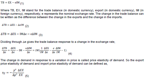
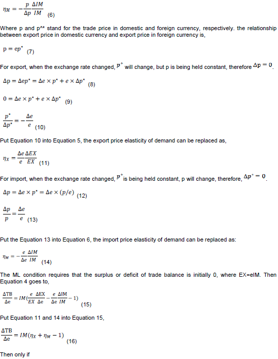
According to the international economics theory, a real depreciation of a country’s currency improves its current account. However, the validity of this assumption depends on a condition called Marshall-Lerner Condition, which states, a real depreciation improves the current account if export and import volumes are sufficiently elastic concerning the real exchange rate. To start with, write the trade balance, measured in domestic output units, as the difference between exports and imports of goods and services similarly measured:
Data
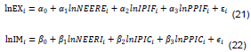
As we all know, the higher the foreign income, the more the demand for export. Therefore, export is a function of foreign income. Alternatively, the import is a function of domestic income, because the higher the domestic income, the demand for foreign goods will increase. Also, competitors’ prices may indeed be correlated with exchange rate changes, because the lower the competitors’ price, the demand for export and import will reduce. Hence, the variables of the export model include Export (EX), Nominal Effective Exchange Rate (NEERE, weighted in export volume), Foreign Industrial Production Index (IPIF), Foreign Producer Price Index (PPIF). The variables of import model include Import (IM), Nominal Effective Exchange Rate (NEERI, weighted in import volume), China’s Industrial Production Index (IPIC), China’s Producer Price Index (PPIC). The export and import model defined as:
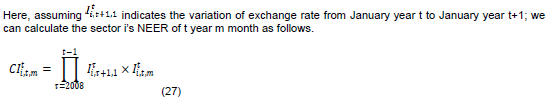
This paper’s purpose is to verify whether the ML condition can be satisfied by using industrial data. It may not be appropriate to use the aggregate NEER published by BIS when calculating the industrial export and import price elasticities of demand, which may cause “Aggregation Bias”. Hence, this paper constructed NEER in 8 sectors (FOOD, MINERAL, CHEMICAL, WOODS, TEXTURE, METAL, EMACHINE, and MACHINE), following the HS code classification; it selected 10 countries and areas (the US, EU, Australia, Canada, Hong Kong, Japan, Korea, Singapore, Thailand, and UK) based on two conditions: 1. They are the important trade partner of China; 2. Their currency is included in the Currency Basket which RMB’s exchange rate refers to. All variables were transformed into nature logarithms. The detailed explanation of each variable is as follows:
(1) Export (EX) and Import (IM). The export data (Total and Sectors, foreign currency dominate), and import data (Total and Sectors, foreign currency dominate) are taken from Wind Database.
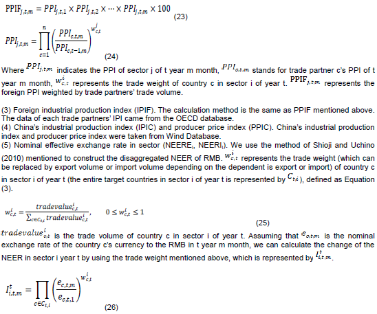
(2) Foreign producer price index (PPIF). This paper obtains each country’s PPI above from the OECD database, and calculates the PPIF as follows:
Pesaran and Shin (1999) provide the ARDL model, which can be applied to a small sample size such as the one used in this study. China’s export and import demand function for the concerned period included 114 observations. While this method provides another advantage to the researchers over conventional co-integration testing, which is even if some variables are I(0), and the rest variables are I(1), a long term relationship between the series can be investigated.
Unit root test
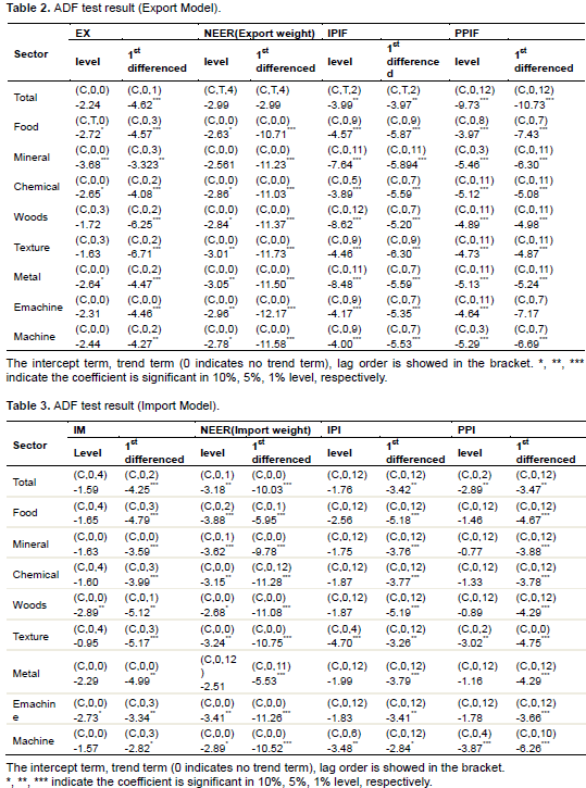
Before estimating the export and import price elasticity of demand, it is necessary to examine the stationarity of all variables, because if the data are unstable, the estimated coefficient may be biased and unreliable. There are several Unit Root Tests to determine stationarity of series or not; and the most popular test is the Augmented Dickey-Fuller (ADF) test. The ADF test results of export model variables and import model variables are given in Tables 2 and 3, respectively.
According to the ADF results, all variables are stationary either in level or after 1st differenced, that is, all variables are either I(0) or I(1). Therefore, the ARDL method was chosen for this analysis.
ARDL bounds test approach
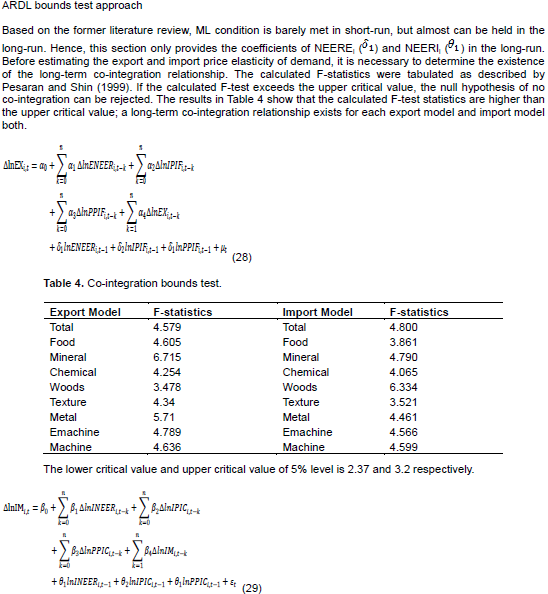
Based on the former literature review, ML condition is barely met in short-run, but almost can be held in the long-run. Hence, this section only provides the coefficients of NEEREi ( ) and NEERIi ( ) in the long-run. Before estimating the export and import price elasticity of demand, it is necessary to determine the existence of the long-term co-integration relationship. The calculated F-statistics were tabulated as described by Pesaran and Shin (1999). If the calculated F-test exceeds the upper critical value, the null hypothesis of no co-integration can be rejected. The results in Table 4 show that the calculated F-test statistics are higher than the upper critical value; a long-term co-integration relationship exists for each export model and import model both.
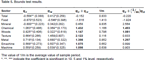
According to the TML condition, whether the movements of exchange rate can adjust trade balance or not depends on the export and import price elasticity of demand. If export and import prices do not lead to a change in demand, no adjustment can be achieved. The empirical analysis tried to investigate whether the sum of China’s export and import price elasticities of demand is bigger than 1 or not. The findings of this study can be interpreted as:
(1) Except for the mineral import price elasticity of demand, the others are significant, which indicates the variation of the exchange rate can affect export or import volume except for mineral. The import of mineral reaches its minimum in 2015, but there is no connection between the drop of mineral import and the RMB’s reform in August 2015. The drop in oil prices, from a peak of 115 dollars per barrel in June 2014 to under 35 dollars at the end of February 2016, is the most important explanation of why China’s imports reduced sharply, also the surplus of trade balance of China reaches its peak in 2015. Hence, the results can barely find the relevance between RMB’s exchange rate and import of Mineral.
(2) Since the export price elasticity of General, Food, and Mineral, and the import price elasticity of Food has a significant negative value, it can be said that both the TML Condition and GML Condition for these industries is not fulfilled. One of the reasons that these industries cannot meet ML Condition is, there is no substitute for these imported products; the price elasticity is extremely low, hence there is limit room for the exchange rate to adjust the prices of these industry’s products.
(3) The export price elasticity of primary goods is bigger than end-products. China’s primary goods only occupy 5% of the total export of China, and do not have competitiveness in the international market. Foreign importers will find other substitutes if the RMB is appreciated or buy more primary commodities from China if RMB is depreciated. But the situation of Chinese manufacturing goods is different. First of all, Chinese manufacturing goods have strong international competitiveness, the demand of “Made in China” would not turn around easily because of the fluctuation of exchange rate; second, exporters in related industries may take several actions to avoid the exchange rate risk, such as sacrifice their profit margin to maintain their overseas market share. These actions of micro-economies may shrink the export price elasticity of demand.
(4) The import price elasticity of primary commodities is smaller than the manufacturing goods. About the import of primary goods, China overwhelmingly relies on foreign commodities plus there are no substitutes in the domestic market, even if the exchange rate fluctuates rapidly, the domestic demand will not change. Therefore, the import volume will stay at the same level. On the other hand, China imports manufacturing goods from overseas, assembles them into end-products in domestic, and export finished goods to overseas. This feature of “Processing trade” let the connection between export and import demand inseparable. When RMB appreciates, the decrease of export demand will cut down the import demand; when RMB depreciates, the import price will increase, then enterprises will use the domestic substitutes instead of using foreign goods, the import demand will lessen.
(5) The results of Texture, Emachine, and Machine meet the TML condition but fail to satisfy the GML condition. The value under GML condition is 0.833, 0.899, 0.903 respectively, which is less than 1 and fails to fulfill the condition to adjust the trade balance. The results not only depict that bigger surplus of trade balance will reduce the value of 1/m; the movement of exchange rate can be hardly used to adjust the trade balance. It also indicates that the TML condition may be ineffective to interpret the correlation between exchange rate and trade balance if a country’s trade balance is surplus at the start.
So far, the study uses the ARDL model to calculate export and import price elasticity of demand for the Chinese economy from January 2008 to June 2018. Going by the empirical results, some industries’ results cannot meet the TML Condition and GML Condition. Rest of the results show the sum of export and import price elasticity of demand that met the TML condition, which assumes that the trade balance is initially 0; but fails to satisfy the GML condition, which assumes the trade balance is not initially 0. If the trade balance is 0 at the very first beginning, there is no need to let the exchange rate fluctuate to adjust the trade balance. The surplus amount of China’s trade balance recorded in recent years has reignited the debate on the effect of exchange rate changes trade flows and global imbalances. Therefore, the results of the GML condition are more appropriate to explain whether the fluctuating exchange rate can influence trade balance.
Overall, the chemical, woods, metal results suggest that GML condition holds in the long-run. This means even though these industries’ trade balance is greater than 0, the variation of exchange rate can adjust the trade balance in these sectors. While the GML condition is not satisfied in Texture Emachine, machine for the sample period data, it indicates that the movement of the exchange rate cannot adjust the trade balance in these 3 sectors. Texture, Emachine, Machine are the backbone of the Chinese economy as they fuel growth, productivity, and employment and strengthen other sectors of the economy. The surplus of these 3 sectors of trade balance occupies 90% of China’s total surplus trade balance in 2018. The empirical results indicate that these 3 sectors’ surplus can hardly be influenced by the fluctuation of the exchange rate, plus the anchor standing of these 3 sectors in the Chinese economy. We may say the appreciation will not succeed in adjusting the trade balance surplus in the Chinese economy.
The movement of the exchange rate was expected to achieve its goal to adjust the trade balance but failed in reality. There are various constraints in which an economy faces macroeconomic factors such as the transition of economic structure, the development of the global value chain, the lessen restriction on trade, and microeconomic factors like the expansion of overseas investment, multiple strategies to avoid the exchange rate risk. As a result, both government and enterprise will take corresponding actions to avoid the exchange rate risk, and ensure the development of international trade. It is much more complicated to convert the trade balance through the change of exchange rate. Therefore, it is not appropriate to expect the trade balance will be transferred to rely on the alteration of the exchange rate.
The author has not declared any conflict of interests.
REFERENCES
|
Ahearn J (2002). Should South East Asia Devalue? Issues in Political Economy 11:1-17.
|
|
|
|
Bahmani M, Harvey H, Hegerty SW (2013). Empirical Tests of the Marshall-Lerner Condition: A Literature Review. Journal of Economic Studies 40(3):411-443.
Crossref
|
|
|
|
|
Bahmani-Oskooee M (1998). Cointegration Approach to Estimate the Long-run Trade Elasticities in LDC's. International Economic Journal 12(3):89-96.
Crossref
|
|
|
|
|
Bahmani-Oskooee M, Niroomand F (1999). Openness and Economic Growth: An Empirical Investigation. Applied Economics Letters 6(9):557-561.
Crossref
|
|
|
|
|
Brooks TJ (1999). Currency Depreciation and the Trade Balance: An Elasticity Approach and Test of the Marshall-Lerner Condition for Bilateral Trade between the US and the G-7. Doctoral Dissertation, the University of Wisconsin-Milwaukee.
|
|
|
|
|
Fang W, Lai Y, Miller SM (2006). Export Promotion Through Exchange Rate Changes: Exchange Rate Depreciation or Stabilization? Southern Economic Journal 72(3):611-626.
Crossref
|
|
|
|
|
Fu J (1997). The Insufficiency and Application of Marshall-Lerner Condition based on its basic Assumptions. World Economy Studies 1:58-62.
|
|
|
|
|
Hooper P, Johnson K, Marquez J (2000). Trade Elasticity for the G-7 Countries. Princeton Studies in International Economics 87:1-72.
|
|
|
|
|
Liang L, Gong Y, Wu F (2019). The 'Deflation Effect' and Sino-US Trade Balance under the Expectation of RMB Devaluation. International Economics and Trade Research 35:50-62.
|
|
|
|
|
Lu Q, Li Z (2013). The Decomposition of RMB Real Effective Exchange Rate and the Revisions of Marshall-Lerner Condition. The Journal of Quantitative and Technical Economics 4:3-18.
|
|
|
|
|
Maura G, Silva SD (2005). Is There a Brazilian J-curve? Economics Bulletin 6(10):1-17.
|
|
|
|
|
Murata Y, Satoma K (1991). The correlation of Japan's Trade Balance and Exchange Rate, the Transformation of Marshall-Lerner Condition. Kansai University Discussion Paper 40(5):863-885.
|
|
|
|
|
Okabe K (2010). The Variation of Exchange Rate and Trade Balance: The Generalized Marshall-Lerner Condition and J curve effective. SFC Discussion Paper, SFC-DP 2010-001.
|
|
|
|
|
Panda B, Reddy DRK (2016). Dynamics of India-China Trade Relations: Testing for the Validity of Marshall-Lerner Condition and J-curve Hypothesis. IUP Journal of Applied Economics 15(1):7-26.
Crossref
|
|
|
|
|
Pesaran MH, Shin Y (1999). An Autoregressive Distributed-Lag Modelling Approach to Cointegration Analysis. Econometrics and Economic Theory in the 20th Century, pp. 371-413.
Crossref
|
|
|
|
|
Reinhart CM (1995). Devaluation, Relative Prices, and International Trade: Evidence from Developing Countries. IMF Staff Papers 42(2):290-312.
Crossref
|
|
|
|
|
Shioji E, Uchino T (2010). Construction of a Goods-group Level Nominal Effective Exchange Rate Data Set and Re-examination of the Exchange Rate Pass-Through in Japan. The Economic Research 61:47-67.
|
|
|
|
|
Thochitskaya I (2007). The Effect of Exchange Rate Changes on Belarus's Trade Balance. Problem of Economic Transition 50(7):46-85.
Crossref
|
|
|
|
|
Zhao M (2005). The Question and Revision of the Marshall-Lerner Condition. Journal of Shanxi Coal-Mining Administrators College 2:106-111.
|
|