The risk problem remains pervasive in the field of Finance. Although Knight (1921) is one of the first to integrate this concept into investment decisions, the modern formulation in the heart of the financial literature is generally ascribed to Markowitz (1952), who suggested that standard deviation (sigma) should be an adequate measurement of total risk or business risk.

However, Sharpe (1964), through his famous Capital Asset Pricing Model (CAPM), proposed beta as a measure of systematic or non-diversifiable risk of financial assets, thus turning the problem into the stock price valuation. This approach consequently shows that the only risk to be taken into account in the explanation of the expected returns is the one related to the market with the underlying assumptions that the market is efficient and that there are no transaction costs. This position is not without criticisms, as one can note that the market is not the only factor to be taken into consideration; and that there is no perfect market in which transaction costs are completely non-existent. It is in response to this criticism that Ross (1976), through the Arbitrage Pricing Theory (APT), proposed that there are several factors of different nature, which must be considered in the explanation of the prediction of stock prices. Fama and French (1993) suggested that one should not neglect the factors suitable for the size and the value of listed companies. Other scholars (Amihud and Mendelson, 1986; Pedersen and Acharya, 2005; Brennan et al., 1998, 2001) proposed the need to take into consideration certain variables suitable for the microstructure of financial markets and more precisely, liquidity in the explanation of the expected returns of financial assets.

Consequently, the investment decisions should not only consider the risk and return, but also the liquidity of the assets concerned. Liquidity, contrary to accounting and banking interpretation, can be seen as the capacity, the ability, or the skillfulness to proceed to significant transaction on shares at lower costs, without any significant influence on the prices of the assets concerned (facilitated transaction). About it could also mean the facility with which an operator in the market finds a counterpart for his operations.

Many studies have been carried out on the American stock exchange market where liquidity and risk are well taken into account in the formation of stock prices but the results are very divergent in other developed and emerging markets. The latter however, presents particular characteristics (they are said to be very narrow, illiquid and quotations are far from frequent there) which offer a good verification opportunity because, according to Hichan (2007), no investor worthy of his name could offer the luxury to be unaware of them. Liquidity is one of the principal factors that should attract investors to the financial market considering the clientele theory (Amihud and Mendelson, 1986). 

Studies in this field has almost left out the African stock market, which however presents rather relevant characteristics, since it is famous for being far from liquid. It is in sense that this study seeks to examine the contribution of liquidity and the associated risk in the explanation of stock price valuation process, in order to draw a set of lessons from it and to compare the results with those found in the context of the American stock exchange market and other developed financial markets.

Moreover, in addition to this contextual and theoretical involvement, one major contribution of this study is essentially methodological. Indeed, it is shown here that the choice stock portfolio panel analysis, makes it possible to reduce the heaviness of the work which is carried out with the standard form of the Fama and Macbeth method like Rahim et al. (2006). More specifically, it makes it possible to cancel the third stage which generally is most tiresome, reducing the number of stage of this method to two either to three.

All theories developed in this approach of the liquidity as explanatory factors of the shares expected returns have a base on the standard pricing models of financial assets. Thus, the two factor model of Amihud and Mendelson (1986) and Liquidity Capital Assets Pricing Model (LCAPM) of Archarya and Pedersen (2005) acted as a base on the Capital Assets Pricing Model (CAPM) of Sharpe (1964), while the four factor model used for the first time by Chordia et al. (1998) before spreading itself largely with this field of research has a theoretical base of Fama and French (1993) model.

 

The two-factor model (The clientele theory)

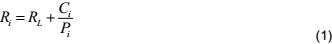
Amihud and Mendelson (1986) suggested liquidity as an essential element of stock price formation process. According to them, a patient investor must profit from an extra return (illiquidity premium) in remuneration of his patience, liquidity being evaluated by transaction costs. The basic idea is as follows: An investor (indifferent from risk), who buys a share and considers possible transaction costs must take them into account at the time he wants to resell. On the basis of this idea, the proposition shows that the required return (rate of return), for an investment in the illiquid assets (I), is given by the output of the investment of perfectly liquid assets (R_L) added to a premium of lack of liquidity represented by the ratio of the cost of lack of liquidity  by the price of the action .

 

 

Equation 1 is obtained under the assumption that investors have a single-period investment horizon. By supposing a multi-period situation, one can generalize this result based on the fact that the price of an asset, which indefinitely offers constant dividends (D_i) is given by the present value of these dividends minus costs expected for lack of liquidity:

 

 

 is the probability of liquidating the concerned asset.

 

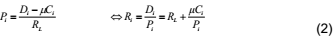
According to Dalgaard (2009), this relation is purely intuitive insofar as it is known that the return obtained on an asset must take into account the expected "liquidity premium". This relation presumes that the investor behaves as the periods of investments were homogeneous. By taking the case of heterogeneity for the duration into consideration, this can be condensed into what is described as "clientele theory", according to which a long-term investor will have a weak frequency of transaction, which will consequently reduce transaction costs (costs of illiquidity) and then allow him to realize a higher output after taking into account the costs relating to it. This simply means that the least liquid assets must be held by the investors over a long investment horizon. Algebraically:

 

 

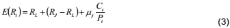
, represents the return required by the investor . This two-factor theory is the basis for other extensions.

 

The four-factor model

Chordia et al. (1998) following the work of Fama and French (1993), proposed a model which makes it possible to take into account the existence of liquidity in the explanation of returns in excess of the risk-free rate for a portfolio of assets. They showed that this exceeds the two-factor model in terms of significance, which explained return more than the CAPM. It is represented in the following equation:

 

 

 is the coefficient which measures the sensitivity return compared to the liquidity. More details on this will be provided in the methodology.

 

Liquidity, illiquidity risks and rate of return required by the investors: a review of empirical results 

Amihud and Mendelson (1986) propose the role of liquidity in financial assets pricing. In their empirical study, portfolios are constituted on the basis of individual systematic risk and value of the liquidity indicator (the bid-ask spread) of the shares quoted on the NYSE from 1960 to 1980. The results obtained allowed them to confirm that liquidity is a decreasing function of the expected returns and also, that this function is concave.

Archarya and Pedersen (2005) use lack of liquidity as indicator to carry out an analysis in 5 steps to show that liquidity and the risk of illiquidity are very significantly taken into account in the explanation of the expected returns of shares on NYSE and AMEX for a period from 1962 to 1995. Also, Datar et al. (1998) used turnover as indicator to test the role of liquidity in the process of stock exchange price formation on the NYSE between July 1962 and December 1991.

The fundamental difference in this study with all the others is that it relates to individual shares rather than portfolio of shares usually used. The method employed is that of Fama and French (1992), taking into account the adjustments suggested by Litzenberger and Ramaswang (1979). The results obtained show overall that the expected return is a decreasing function of liquidity. More precisely, it is positively and significantly related to turnover contrary to the indicator of illiquidity which must be negatively related to return with respect to the Amihud and Mendelson’s (1986) clientele theory.

Chordia et al. (2001) study the effect of variation of liquidity on the output of shares quoted on the NYSE and the AMEX from January 1966 to December 1995. According to them, insofar as the relation makes a consensus in the literature, investors should protect themselves from the risk related to its variation, since they are supposed to be risk averse. The empirical method used is that of Brennan et al. (1998), which binds the expected output to volatility or liquidity. The results show that the effect of liquidity measured by turnover and the ratio of lack of liquidity on the output is significant and persistent, which means that return is a decreasing function of liquidity in the American financial market.

Chan and Faff (2005) highlight the role of liquidity in the financial valuation of assets by increasing an explanatory variable relating to liquidity. The technique used is that of Fama and French (1993) and the monthly data used relates to the shares quoted on the Australian market over the period 1989 to 1998.

The empirical analysis shows that liquid assets ratio is significant just like on the American market. This means that, the turnover tends to have an effect on the expected returns of shares. Moreover, they show that the least liquid shares tend to have significantly positive beta while the most liquid portfolios tend to have negative betas. These results are robust and are consistent with financial literature on the American market.

The object of the work of Soosung and Lu (2005) is to give an insight on the role of the liquidity risk in the explanation of the expected return of shares on the British stock exchange market. Particularly, they seek to check if the liquidity or the value of the liquidity premium is well taken into account as on the American market. They use variables of the model of Fama and French (1993), and the indicator of liquidity of Amihud (2002) over a period of study from January 1987 to December 2004. The results show that irrespective of the strategy of portfolio formation, large companies are more powerful than the small ones and the direction of relation between return and liquidity is contrary to that highlighted in the literature, although the latter is taken into account on this market. That is true whatever the test of robustness carried out.

Shing-Yang (1997) examines the problem of measurement of liquidity and its impact on the surplus of expected return of shares on the Tokyo Stock Exchange between 1975 and 1993. The results show that the stocks which have a raised turnover tend to have a weaker expected return (adjusted with the risk). Also, Geert (1998) studied 1700 shares of a group of 20 emerging stock exchange markets over the period of 1975 to 1997. The measurement of liquidity used is the turnover and the other explanatory variables are those of Fama and French (1992). He finds out that the liquidity is strongly related to the expected return in excess of the risk free, but that it is very unlikely that this is taken into account overall on these markets.

Furthermore, Bekeart et al. (2007) show that liquidity becomes one of the most significant factors in the stock exchange prices formation process of the 19 emerging stock exchange markets, contradicting more or less the results of Hearn and Piesse (2005), and Hearn (2007) on Africa in the South of Sahara.

These results aligns with those of Huson (2009) on the Malaysian stock exchange market, Dalgaard (2009) on Denmark, Barend (2009) on the South-African market and Miralles et al. (2011) on the Portuguese market, in that, although liquidity is a significant factor in the stock exchange price formation process, the pricing of the associated risk is long in becoming a reality

Source of the data, selection of the variables and portfolios formation

The data

Data used in this study are obtained from the financial database of BRVM. They are primarily the data on the daily transactions and those on the annual financial statements of the companies quoted at the BRVM. After several filters, in particular with regard to the incompleteness and the absence of information, a sample of 32 titles is retained for one period which extends from 1998 to 2008. It should be noted that it concerns particularly the 32 most traded shares on this stock market during this period. It should also be noted that the study use the average value of information (the monthly average price of share) over the period considered, which is more representative.

 

The variable of the study 

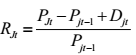
The explained variable is the return in excess of the risk free rate . The return of portfolio i is a simple average of that of the individual shares which constitute it. It is calculated according to the method suggested by the CAPM, while taking into account the net dividends produced by each share, as seen below:

 

, with n being the number of share in a portfolio i.

 

, measures the profitability of share j at

 

time t  represents respectively the price and the dividend of share j at time t).

The risk free rate  used is the interbank rate, because the public treasury bonds rate (in one year) regularly used in the literature is very unstable and irregular in the UEMOA zone. The use of the simple averages (arithmetic mean) contrary to the weighted averages joined the works of Amihud and Mendelson (1986), Amihud (2002) and Chordia et al. (2001). The reason is simple: In theory, the use of weighted averages makes it possible to take into account the size effect of large companies which could skew the results, but that is already taken into account when using stock exchange capitalization (book to market) as explanatory variable.

For the explanatory variables, we use the three variables suggested by Fama and French (1993). It concerned the return of the market portfolio in excess of the risk free rate (R_Mt – R_f). One of the problems in the determination of the market portfolio is that it must be the most possible representative. To face this problem the study used the BRVM composite index which represents the whole securities quoted on the BRVM. The market portfolio return is the same as that in the CAPM, being the ratio of the difference between the value of the market index () between two consecutive periods, by that of the previous period:

 

 

The size of the company or the portfolio here makes it possible to take into account the "the size effect", which supposes that the large companies or large portfolios will have higher returns as long as their sales are high. This effect is taken into account in this study by the stock exchange capitalization (CB), which is the product of the number of title j held at moment t and the stock exchange average price of this same security over the same period.

 

 

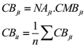
 respectively represent stock exchange capitalization, the number of shares held and the average price of the share j during the month t.

In line with the study of Amihud and Mendelson (1986) and Batten et al. (2010), the value of stock exchange capitalization used is log-normalized to take into account the imperfections of the market.

The "book to market" (BM) takes into account the variations of the company. It is about the relationship between two values of the company: The book value (VC) and the market value (VM) for share j at time t:

 

 

To obtain the value of the BM for a portfolio, it is enough to make the simple average of these individual values for the shares which make it up in the month considered. 

The study used not only one measurement of liquidity, but also an indicator of lack of liquidity. Several studies used the "bid-ask spread" as an indicator of lack of liquidity but on most emerging stock markets like the BRVM, one cannot have the required information for its determination because a system of order and not of price quotation is still being used. It is for this simple reason that other indicators like the turnover or the ratio of illiquidity are used here to measure liquidity.

Datar, Naik and Radcliffe (1998) proposed Turnover (TO) as a measure of liquidity to mitigate the insufficiencies of the "bid-ask spread". For them, it is the ratio between the volume of transaction of the title (j) during the month t by the number of title held or available during the time and it is given by:

 

 

, respectively represent turnover, volume of transaction and the number of securities held for stock j during month t. To calculate the turnover of a portfolio (i) of security (j) simply involves making simple average of the turnover of shares included in the portfolio. There are several advantages to use the turnover as an indicator of liquidity. According to Xuan et Batten (2010), it has a very strong theoretical attraction; Amihud and Mendelson (1986) showed that at equilibrium, the return is correlated with the transaction frequency.

Thus, if one cannot directly observe the liquidity by the bid-ask spread, that can also be done in an effective way with turnover. In second place, the turnover is one of the most easily calculable measurements, if one takes into account the system of functioning of emerging stock exchange markets in general, and the BRVM in particular. It is supposed to be a decreasing function of the expected output. Due to the various difficulties that arise in the evaluation of liquidity, Amihud (2002) proposes an indicator, which can readily be obtained at the emerging markets and this has gained a great importance in the literature. It is presented in the form of a relationship between daily return of asset j in the month t of year n by the volume of corresponding transaction (in value). Nevertheless, this indicator is slightly modified (without changing its direction and its significance) in that instead of working with daily data as, we rather used monthly values. Algebraically one can write:

 

 

 respectively represent the ratio of lack of liquidity, the output and the volume of transaction for each title j in the month t of year n.

 

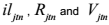
Each one of these variables are calculated for each individual stock before being aggregated on the level of the portfolios. The portfolio of stocks are used as against individual stocks simply because this process makes it possible to reduce skewness in the estimate of the explanatory variables. Just like in Fama and French (1993), we form six (6) portfolios according to a double assignment. The method of formation adopted is similar to that of Amihud and Mendelson (1986) and Dalgaard (2009) with regard to the technique and the proxies of formation of stock portfolios. Initially, the 32 BRVM’s shares are classified according to the decreasing value of their liquidity then divided into three groups by considering the thresholds of 30% and 70%. In the second time, each one of these three groups is segmented into two equal partitions compared to the value of beta of each stock constituents of the portfolio. Beta used is obtained from the regression of market model of Sharpe (1964).

Finally, there are six (6) portfolios as presented in Figure 1 below. A particular attention is also given to the period of study because it can rather be special in the methodology of Fama and Macbeth (1973), in the sense that it gives the possibility of being broken up into sub-periods with an aim of not only making the model more predictive but also of making the results more significant and better in explaining the phenomenon studied. Typically, with the present case and in reference to the literature on this methodological approach, our period of study which is 10 years (1999 to 2008) is subdivided in two sub-periods: one estimated period (of the betas for each explanatory variable), and a test period which will make it possible to estimate the factors of sensitivity to be used to explain the studied phenomenon (gammas).

 

 

Thus, the first four years (1999 to 2002) are used to estimate the betas and the last six (2003 to 2008) years to estimate the gammas.

In addition, in order to obtain the most significant and representative possible results of the sample, the beta of Sharpe’s market model which is used for the formation of the portfolios is calculated for each title on the whole for the period of study^[1].

The comprehension of all these processes and techniques of analysis is easier when these variables are specified in an econometric model.

 

The econometric specifications

It will be necessary to distinguish the econometric model, which makes it possible to detect the role of the liquidity from what makes it possible to take into account the risk of liquidity in the explanation of the expected return of stock portfolios.

 

The role of liquidity in the stock pricing process

To detect the role of liquidity in the explanation of expected return, we go through the following procedure:

Firstly, we regress with ordinary least square for each portfolio i, each month t, using the following model:

 t= 1, … , 49

For each portfolio i one estimates each month as from January 2003, the parameters Each one of these parameters is obtained by making the regression of the preceding model on information from the previous 49 months. The estimated value of a parameter at January 2003 is obtained from the regression of the preceding model using data from January 1999 to January 2003. The objective of this first regression (over period of estimate) is to obtain the monthly value of the bêtas () of each company characteristic, which will be used at the second stage to explain the role of liquidity in the explanation of the return of the portfolios of shares.

Secondly, the factors of sensitivity  obtained by the ordinary least square are used simultaneously with the liquidity in a panel of six portfolios. ¶The model at this second phase becomes:

 

 

t= 1, …, 72 et i= 1,…, 6 (Model 1)

LIQ represents the liquidity variable which is measured either by turnover or by the ratio of illiquidity.       

At this level, because instead of individually making the regression for each portfolio before aggregating thereafter the results at the level of the overall market, we choose a form of regression^[2] which makes it possible to make both in one, while reducing the risks of omission and calculation which can affect the stage of aggregation of the results in the procedure. This second regression (which makes it possible to really explain the studied relation) is made on all of the test period, which extends from January 2003 to December 2008. The indicator of liquidity (turnover or ratio of lack of liquidity) used for each portfolio is that of the preceding period (month); the use of the indicator of liquidity of the previous period aims to make the model more predictive.

The first gamma  does not represent anything theoretically and must however be null. The 3 gammas following  represent the risk premiums and consequently must be different from zero according to the relation which exists between liquidity and expected output. The last gamma  represents the effect of liquidity in the explanation of the excess expected return, the awaited sign of this relation is a function of the indicator used. If it is about a measurement of liquidity like the turnover, then the relation should be negative since the less liquid a portfolio is, the higher is the required return. If on the other hand, the indicator used for the liquidity is an indicator of lack of liquidity then the awaited sign becomes positive.

 

The illiquidity risk and the stock price formation process: the model

In this work, in addition to the direct pricing effect of liquidity on the return of individual shares, we analyse the relationship between liquidity risk and return of portfolios of shares on the BRVM. To evaluate the impact of liquidity in the explanation of expected return, its value is introduced at the second stage of methodology. Now, when we want to check if the associated risk (risk of liquidity) is priced, this one is introduced at the first stage, such that a beta value is also calculated for the liquidity variable. Just like previously, the analysis is done on portfolios of shares instead of on individual shares.

The first regression which makes it possible to obtain the factors of sensitivity is made for each portfolio i at the moment t, according to the following model:

 t = 1, … , 49

As previously mentioned, the model from the first stage already integrates liquidity which is consequently considered as a risk and no more in terms of degree (level of liquidity). Thus, the sensitivity of the return to the changes in liquidity is the time taken into account at the first stage of the regression (Fama and Macbeth, 1973).

Then, the whole of the parameters of the portfolios obtained at the first stage (factors of sensitivity ) are used in the regression as follows: 

 

 

t = 1, …, 72 and i = 1,…, 6 (model 2)

The regression parameters are the risk premiums, which explain the disclosure of the risk of each portfolio. So the portfolio with a high sensitivity on one or the other of the four factors, must expect the highest return in theory to remunerate the additional risk to which it is exposed.¶ This is verified and is simply perceptible in the CAPM where portfolios of shares which are most sensitive to the variation of the market variable (shares with high beta) are supposed to have a higher return.

In short, the method used here is that of multiple regressions in the first phase and panel analysis in the second phase (that enables us to check the sense of the relation between liquidity and return). More clearly and simply, one first estimates by the ordinary least square method the betas or factors of sensitivity for each variable which is supposed to explain the expected return of the portfolios of shares and in the second time, one estimates the gammas by the panel regressions.

Pre-test and post-estimation tests were carried out to ensure the robustness of the estimates. These include, among others, Breitung (2000) unit root tests to account for stationarity, Breush-Pagan test to account for heteroscedasticity and Hausman test to account for fixed and random effect of the various panels respectively.   

At first, estimate of the factors of sensitivity is focused on the 3×2 liquidity-beta portfolios but this can appe0r skewed and less specified. For this reason, to check the significance of the results, same work is restarted for portfolios formed starting from beta of shares only. Still aimed at checking if the liquidity and the associated risk are significant factors in the explanation of the expected return, the variables of Fama and French are removed from the model and, on the other hand, in line with the Mooradian (2010) model, the two indicators of liquidity are simultaneously used in the same model. The objective is not to make the model more or less explanatory but, simply to check if the relation between liquidity and return remains unchanged when the model loses or gains power. Again, in order to take into account the January effect, information on the first month of the year is eliminated for each portfolio of the study.

 

The descriptive statistics

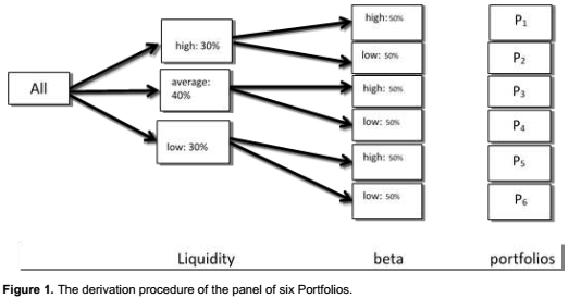
Here, we analyse the relationship between return and liquidity using the average of the observations according to each portfolio formation method. The same process is repeated with correlation coefficients between the various variables of the study and according to the various methods of portfolio formation. Table 1 brings out the average of each liquidity variable  and return in excess of the risk-free rate. From this table (3X2 TO-beta portfolios), one can note that while the average value of the market return adjusted with the associated risk isle negative (approximately -4,5%), the return adjusted to the risk of all the portfolios is completely positive and varies between 1,6418% for portfolio 4 (P4) to 10,8725% for portfolio 2 (P2). These values confirm the assumption of a strong variation and very high value of the returns on the African emerging stock exchange markets globally, and on the BRVM in particular. Moreover, it is equally noted that Sharpe’s theory of risk premium tends to be respected, because the first three portfolios, which are the riskiest are also most profitable. Also, portfolio 2 that has the highest liquidity value measured by the turnover (TO = 0,004620) has the highest output (0,108725). But, portfolio 5 which has one of the three lowest returns is the least liquid on average. This leads s that return and liquidity (turnover) move in the same direction. The pace of this relation is confirmed even more when it is noted that the three most liquid portfolios are also the most profitable. In addition In addition, it is clear in terms of the average values that liquidity is an increasing function of the output of stock portfolios quoted on the BRVM.

 

 

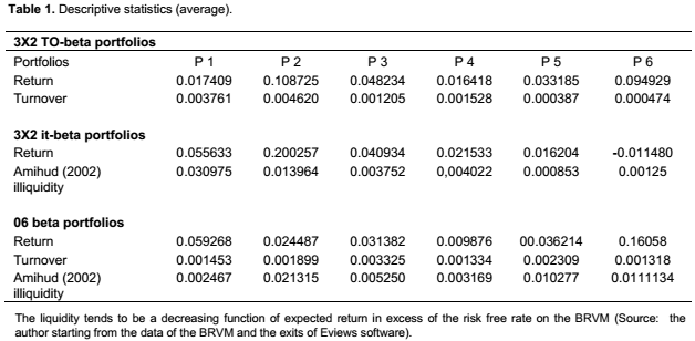
Table 2 shows that the result almost does not change when the indicator of lack of liquidity is used as proxy. More specifically, the two least liquid portfolios on average (P₁ = 0,030975 and P₂ = 0, 013964) are most profitable (P₁ = 0,055633 and P₂ = 0, 200257). Additionally, starting from the second portfolio, the average output decreases gradually until the sixth. However, the method of formation of the portfolios shows that lack of liquidity decreases from P₁ to P₆. Thus, P₆ would be most liquid; this is confirmed owing to the fact that the last two portfolios (P₅ and P₆) hold the lowest average values of the ratio of illiquidity and consequently are most liquid. And also, by the fact that the more the portfolio is profitable, the more the average value of the ratio of lack of liquidity is decreasing.

 

 

For the third method of formation of the portfolios (Table 3), the results are almost identical, but since the two variables of liquidity are at stake here, it is noted that the more the average value of turnover (TO) increases, the more that of the ratio of lack of liquidity (IT) decreases for all the portfolios. This proves that these two variables move in opposite directions.

 

 

From the foregoing, it is clear that liquidity is well taken care of on the BRVM and the related risk is priced. In other words, liquidity would be a decreasing function of the output because on average, the most liquid portfolios are the least profitable. The analysis of the correlation coefficients between the variables shows us a set of results:

 

1. The Sharpe’s variable appears to be the most significant variable in the explanation of the expected return, since it has the highest correlation coefficient (between 18% for P₂ and 57% for P₃), which respects the

Sharpe principle in particular, with regards to the direction of the relation.

2. The relation between the expected output of the portfolio and the variable which takes into account the size of the company in the model (stock exchange capitalization (CB)), is positive overall irrespective of the method of formation of the portfolios. This shows that in theory, the larger the firm the more significant will be its expected return. This analysis is against the results of Fama and French (1992, 1993). According to the latter, the shares with weak stock exchange capitalization must profit from a greater risk premium related to their size. In our case, this result is obtained only when the portfolios are formed from the individual betas of shares.

3. The Book to Market (BM) variable which takes into accounts the valuation of the firm whose share is quoted, is for most portfolios negatively related to the expected return adjusted to the risk. This consolidates the results of Fama and French (1992, 1993).

4. Regarding liquidity, the turnover, in spite of some contrary tendencies, presents a negative relationship to the expected return. On the contrary, the relationship to the liquidity measured by the ratio of lack of liquidity completely respects the literature, since the expected return of the portfolio is an increasing function of lack of liquidity. This clearly respects for almost all the portfolios whatever the method of their formation. Important information that is provided in this matrix concerns the relation between the two liquidity variables. For Mooradian (2010), the direction of the relation is negative when they are of different nature. But in the case of BRVM, this relation varies in a negative way between 0, 06% and 18%.

In conclusion, these statistics enable us to say in advance that the illiquidity risk correctly appears to be priced on the BRVM.

 

The liquidity role in stock pricing process

After the various corrections recommended by the results of the econometric tests we seek to detect the place of the liquidity factor in the explanation of the expected return by estimating Model 1. The results are a function of the variable of liquidity used.

 

The turnover as an indicator of liquidity

To evaluate the contribution of liquidity (measured by turnover) in the pricing of stocks, the regression of the regression of Model 1 are presented in the following table: One can note that all the gammas have the expected signs but only three are significant including the constant . This last is significant at 1%, a proof that even if the model is overall significant at 1%, certain variables must be omitted in the explanation of the expected return on the BRVM. ThisTt This does not respect our expectations (it was supposed that constant is null), but is significantly in line with Ross’s (1976) work on the existence of a non-quantifiable number of factors to be taken into account in the shares (portfolios of shares) return forecast. In addition to the constant, the other gammas respect the underlying assumptions. The value of the coefficient which explains the relation that exists between the expected return of portfolio i and the return of  the market is approximately 0, 2%. This means that a 1% variation of market return engenders a variation in the return of the shares for about 0, 2%. This value very weak as the parameter is not significant. But if it should be left within the meaning of the relation, it will be said that it is in agreement with literature like the work of Sharpe (1964) and Saud et al. (2013) on the Iranian stock exchange market.

The coefficient , which takes into account the size of the company belongs to one of the significant parameters of Model 1. In fact, the value (absolute) of this parameter is equal to approximately 11, 1% and is significant at 1% (P > |z| = 0,003 < 1%). This means that the risk related to the size of the company is recompensed on the BRVM. This result simply shows that the companies which have a market value tend to be the least profitable. Fama and French (1992, 1993) found the same result on the American market, just as Miralles and al. (2011) on the Portuguese market and Saud et al. (2013) who showed that this relation is significantly negative (at 1%). On the other hand, Molay (2002) finds contrary results to those of Fama and French (1992, 1993) not only for the size of the company, but also concerning the "Book to Market" which takes into account the value of the listed company.

Another significant parameter in the explanation of the BRVM’s expected return on stock portfolios is that which takes into account the risk related to the correct valuation of the company . An increase by 1% of this factor is at the origin of an increase of approximately 20% on expected return in excess of the risk-free rate. Several authors found this same result which had first been proposed by Fama and French (1992). For instance, Miralles et al. (2011) find that contrary to stock exchange capitalization (market value), risk related to the market value is an increasing function of the share portfolios’ return. Saud et al. (2013) found that the value of the parameter  is very high compared with that of . Also,alsoA Molay (2002) and Mourina et al. (2012) show that this relation is rather opposite with the results of Fama and French (1992, 1993).

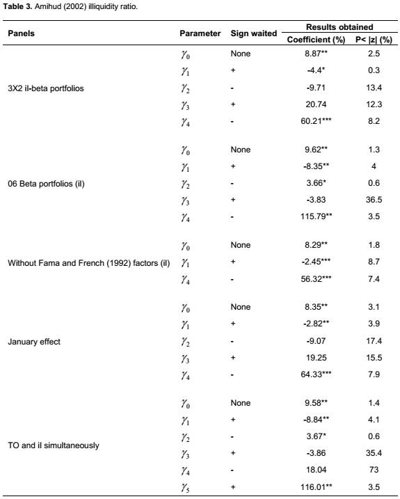
Lastly, gamma estimates  which is that on which this study is based has a negative value. This value is highest in absolute terms among all the gammas of the model. For an increase of 1% of the level of liquidity of the portfolios of shares, there will be a reduction of more than 100% of the expected return. It is the only phenomenon that is non-significant. Nevertheless, as regards the direction of the relation between liquidity and expected return in excess of the risk-free rate, it respects existing results in that liquidity is a decreasing function of output.

Thus, the most liquid shares are the least profitable; agreeing with the clientele theory such that investors who prefer the most liquid shares are short-term investors. One can consequently say that even if the significance is not verified (we can even see that P >|z| is just slightly higher than 10%), it appears that the BRVM stock market takes into account liquidity when it is measured by turnover. These conclusion is in line with Datar et al. (1998) who found that expected return is significantly and negatively related to the liquidity measured by turnover on American stock market. For them, this result is robust even in the absence of Fama and French’s (1993) variables.

Batten and Xuan (2010) also find the same type of relation between liquidity and return on a set of emerging stock exchange markets. Soosung and Lu (2005) found a contrary result on the British market, although the significance is not verified.

These results do not change with the various tests of results’ robustness, except liquidity which becomes significant at 10% level when the January effect is taken into account, an indication that BRVM is affected when January information excluded. Thus one can say that even if its significance is long in coming, the turnover is by far the most significant factor (with more than 100%) in explanation of the expected return of the BRVM‘s equities portfolios.

 

The illiquidity indicator

Amihud’s (2002) illiquidity indicator 

By replacing turnover in Model 1 with illiquidity ratio, the results provided in Table 5 are more precise with regards to the role of liquidity in the stock price formation process.

More specifically, the constant term, the market portfolio return, the company size and the book to market value respectively, did not change sign. Only that their significance varies from one panel to another. On the other hand, the importance of liquidity becomes more visible in the sense that its effect is at 5% significant when the two indicators of liquidity are simultaneously used in the same model and 10% everywhere else. The January effect is also significant when one takes into account lack of liquidity.

However, in spite of some disturbances, when liquidity is measured by turnover, it is well taken into account in the BRVM’s stock portfolios price formation process (more than 100% with TO and nearly 60% with Il). The interrogation which persists consists of knowing if the risk which is attached there is also priced.

 

The illiquidity risk in the stock exchange price formation process

Just like in the preceding section, the study has the results for each indicator of the liquidity.

 

The turnover as measures of the illiquidity risk

Table 4 shows the results when is used in Model 2 as a measure of risk. The constant is always significant at 1% level in whatever panel that is considered. The market variable (beta) has a negative coefficient  of 1, 10% and is not significant. This simply implies that if it varies by 1% the expected return of the portfolios of shares will vary in the opposite direction by 1, 10. Thus the most profitable stocks are the least risky, which means that the systematic risk (market return) is not priced on the BRVM within the Sharpe framework. This result is normal given the characteristics of the emerging stock exchange markets where returns are notable to be strongly volatile and most listed companies are very weak para-public and public companies.

 

 

 

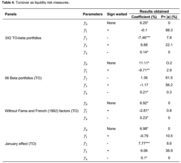
The risk related to the company size  has a negative value (7, 46%) and significant at 10% (P > |z| = 0,078 < 10%). An increase by 1% in the size of the BRVM’s listed companies leads to a reduction in its return by 7, 46% per month, which corresponds to an annual remuneration of 1,371^[1] per unit of risk.

Consequently, the risk related to the size of the company is well rewarded by the threshold of 10% on the BRVM. These conclusions contradict the work of Molay (2002) on the French market and of Lu et al. (2005) which show that large companies are more powerful than smaller ones.

The risk related to the value of the company  is positive (6.88%) but not significant since its p-value is higher than 10% threshold. This positive sign is the expected sign since it supposes the risk premium associated with the company’s value is consistent. The increase in the value of the company (either by reduction of the number of shares without there being as much reduction in the book value, or by raising of prices of the shares) is priced by an increase of 6,88% in a monthly expected return in excess of the risk-free rate. These results are consistent with the analysis of Fama and French (1992, 1993), of Chordia et al. (2001) on the American market and that of Beert et al. (1998) on a group of 20 emerging stock exchange markets.Financial literature (Chordia et al., 2001 and Datar et al., 1998) suggest that for a liquidity risk (evaluated by turnover) to be priced in a market, it would be necessary that the relation between it and the expected return should be negative. The results in Table 4 rather show the opposite. In fact, the value of the premium  is positive (0, 14%) and significant at 1%. This is a proof that increase of a share’s liquidity risk (of 1%) will rather lead to a reduction in the expected return approximately by 0,14%. Thus, the relation between liquidity measured by turnover (TO) and the yield are positive: risk of liquidity is not recompensed on the BRVM. The investors who prefer to hold long-term shares do not receive remuneration on the additional risk which they support; on the contrary, they lose their surpluses of profitability. This contradicts the "buy and hold" strategy recommended to investors on the emerging stock exchange markets.This result is also contrary to the work of Datar et al. (1998) and that of Chordia et al. (2001) on the American market. But is in agreement with those of Nahandi et al. (2012). Miralles et al. (2011) also find that the most liquid shares in Portugal are most profitable. Illiquidity risk is thus not priced with turnover even when Fama and French’s (1992) factors and January information are excluded, or even when the two liquidity indicators are simultaneously used.

 

 

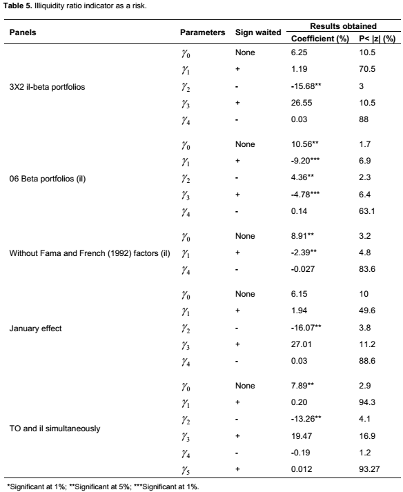
The illiquidity ratio as a risk measure

 

From Table 5, risk premium which is related to the market portfolio  has become positive such that at a non-significant level (P > |z| = 0,705 > 10%), an increase in the market risk is priced by an increase in the portfolio’s return considered by about 1.19% per month, for an annual premium of 15.25%^[2]. This is an indication that illiquidity is considered better on the BRVM. This may be considered normal since African markets are famous for being largely less liquid. The systematic risk related to the company size is better remunerated on the BRVM in that the value almost doubled compared to the case where the TO is used (15, 68% against 7, 46%). The pricing  of "risk-size" is also significant at 5% against 10% previously. This once more shows the effectiveness of the ratio of lack of liquidity compared with turnover on the BRVM. As regards the risk premium attached to the company value , it is significant and its value doubled considerably with the same conclusions. With regards to liquidity risk, certainly lack of liquidity is slightly an increasing function of expected return in excess of the risk free rate (0.031%) but not significant contrary to expectations. A reduction of liquidity by 1% leads to an increase in expected return of about 0.031% per month or 0.37% per annum. This result in sharp contrast to the value of liquidity premium (4.6%) found by Acharya and Pedersen (2005) and 1% by Amihud and Mendelson (1986) in America. On the emerging markets, Dalgaard (2009) found a monthly premium of 5.9% in Denmark. This shows the weak liquidity of the African financial markets. Thus, in spite of the multiple tendencies which seek to contradict the basic results in particular when turnover is used as indicator of liquidity, we do not have enough proof for saying that liquidity risk is priced on the BRVM. Only the risk related to the size seems to be.

 

In conclusion, the use of portfolio panels in the estimation method enabled us to conclude that although liquidity is one of the most significant factors (or most significant according to our results), the risk associated is not priced on the BRVM. That means that apart from risk and profitability, liquidity must be given due consideration in the stock market’s investment decisions. A possible explanation is directly linked to the principal characteristic of the African stock exchange markets with propensity for inefficiency. Another conclusion from our comparative analysis is that each financial market, except those of American market, has its own specificities with regards to the concept of liquidity. It then becomes imperative to set up policies that will support efficiency of the emerging stock exchange markets or those that will reduce its inefficiency.

We document a strong instability of turnover as indicator of liquidity. This casts a doubt on its explanatory power. A new research track would be to seek to know which indicators of liquidity could be adapted as suitable to emerging financial markets overall and Africa in particular; or, if it is possible, to create an indicator that is specific to the African continent.

In addition, of all the traversed literature, none treats of the applicability of Archaya and Pedersen’s (2005) model of liquidity on African stock exchange markets. This new question could also be subject to a new study, aimed at checking if the African markets have specificities compared to this theory.

Finally, we note that when the portfolios are formed on the basis of individual share betas, the results become very unstable.

The authors have not declared any conflict of interests.