Forests are important in the lives of local communities as they provide poles for construction, wood fuel for cooking, help reduce soil erosion and provide various foods and medicines due to biodiversity. Most local communities depend on forests in supplementing their livelihoods. At the moment, forests are being lost and it is important to understand the impacts of the lost. Therefore, the objective of the study was to provide a holistic evaluation of the impacts of deforestation on ecosystem services in Kamfinsa sub-catchment of Kitwe in Zambia. Loss of forest biomass, biodiversity, and soil erosion were key proxy variables for loss of ecosystem services. Geographical Information System (GIS) and Remote sensing techniques were used to assess the impacts on the ecosystem. The results showed that deforestation reached 576.3 ha per year during the period studied. The forest loss corresponds to an emission of 43.73 ton of carbon per hectare from above and below ground biomass valued at US$243.60 per hectare. According to this research soil erosion risk assessment, 1.59 ton of soil was lost per hectare per year, equivalent to US$ 57.20 loss per hectare. The indigenous forest cover reduced from 13,430.5 ha (1990) to 2,904.7 ha (2010), with a corresponding change in NDVI index for loss of forest vigor and biodiversity of 0.56 and 0.32, respectively. The major forest loss occurred from indigenous forests. The study has shown that deforestation in Kamfinsa sub-catchment area calls for the urgent promotion of an integrated and comprehensive approach to addressing the drivers of deforestation to ensure continued supply of ecosystem services.
Ecosystems drive the primary environmental cycles such as the continuous circulation of water, carbon, and other nutrients. The water, food and raw materials needed for human livelihood security originate from the ecosystems surrounding human settlements (Falkenmark, 2003). According to Digest (Evans, 2005), human activities have modified these natural cycles, especially in the last 50 years by increasing their freshwater use, carbon dioxide emissions and fertilizer use, which has affected the eco-system's ability to provide benefits to humans. Historically, the nature and value of earth's life support systems have largely been ignored until their disruption or loss highlighted their importance (Evans, 2005).
There is much interest in valuing the totality of ecosystem services (Costanza et al., 1997); however, such estimation of the total financial value of ecosystem components and services is difficult and may not mean much to the management of ecosystems (Pearce and Pearce, 2001). The appropriate context for economic valuation is, therefore, the value of a small or a discrete change in the provision of goods and services through, say, the loss or gain of forest cover (Secretariat of the Convention on Biological Diversity, 2001).
Deforestation has recently revealed the critical role forests serve in regulating the hydrological cycle through the mitigation of floods, droughts, the erosive forces of wind and rain, and silting of dams and irrigation canals. Forests are one of the most important terrestrial biomes contributing immensely to carbon (C) sequestration and storage, as well as regulating other climate related cycles (Kalaba et al., 2013). Some primary threats associated with land use change include a loss of biodiversity and carbon, nitrogen, and biogeochemical cycles disruption; human-caused invasions of exotic species; releases of toxic substances; possible rapid climate change; and depletion of stratospheric ozone (Daily, 2000).
In recognizing that farmers are key managers of most productive lands on earth (Dale, 2007), this study quantified the impacts of human activity on ecosystems services by focusing on forest loss, soil erosion, and biodiversity. The approach aimed at enhancing the understanding of the dynamics between environment, economic and social dimensions. Integrated Water Resource Management offers an opportunity to take a comprehensive approach to human livelihood security and protection.
According to UNCCD (2012), land degradation is a reduction or loss, in arid, semi-arid and dry sub-humid areas of general biological or economic productivity or complexity of rain-fed and irrigated land under crop, rangeland, pasture, forest, and woodlands. This result from a process or combination of processes, including human habitat and land use, soil erosion caused by the wind and water; degradation of the physical, chemical and biological or economic properties of soil; and long-term loss of natural vegetation.
To understand the dynamics and the cost of soil degradation to enhance planning for ecosystem services management, a holistic approach is required, especially as regards decision-making. Sectoral decision-making is indeed one of the major causes of land degradation when various economic benefits provided by multifunctional agricultural landscapes and natural ecosystems are not considered (Hein, 2009). Knowledge of the nature of land use, land cover change and configuration across all spatial and temporal scales is a prerequisite for sustainable environmental management and development (Turner et al., 1995).
It is important, therefore, to assess the impact of deforestation on ecosystem services as it will provide information to enhance the planning process. A wide range of social, institutional, and economic factors play a role with regards to the lack of sustainability in the management of natural resources (Lambin et al., 2003).
Hydrology has often been the domain of engineers focusing on river flow phenomena of societal relevance while ecology has been the domain of biologists with a focus on climate/ecosystem dynamics (Falkenmark, 2003). The weak governance associated with water resource development, particularly a single-minded, engineering – economic approach to the ecosystems services, has led to significant social and environmental impacts disproportionately affecting the rural poor that rely on function of water ecosystem (IIED, 2007).
Agriculture is a key driver of the global economy; however, the primary challenge is to simultaneously secure enough high-quality agricultural production, conserve biodiversity and manage natural resources, as well as improve human health and well-being for the rural poor in developing countries (IUCN, 2008). The socio-economic and physical factors which drive soil erosion, therefore, need to be addressed in tandem (Boardman et al., 2003).
Zambia, with a population of about 17 million people, is endowed with a variety of natural resources with a total land area of 752,000 km2. The country’s forest cover is estimated at 49.9 million hectares or 66% of the total land over of Zambia (GRZ, 2009). The total biomass (that is, above and below ground) is estimated at 5.6 billion tons, with additional 434 million tons of dead wood biomass; for a total biomass estimated at 6 billion tons of this biomass, there are approximately 2.8 billion tons of carbon stored in the forests (GRZ, 2009). About 50% of the domestic honey trade is consumed by rural population, 36% is sold to traders, 8% is sold on the roadside and 6% is traded in urban areas. In 2003, Zambia exported medicinal plants valued at an estimated US$ 4.4 million (Ng'andwe et al., 2006).
The forestry sector in Zambia contributes about 6.3% to the GDP (Turpie, et al., 2015). The total renewable water resources of Zambia amount to about 105 km³ per year of which 80 km³ are produced internally (World Bank, 2010) Average per capita fish supply has declined from over 11 kg in the 1970s to approximately 6.5 kg in the 2000s (Musumali et al., 2009). According to the GRZ (2011), wildlife resources range from birds and reptiles to mammals. There are about 733 bird species (76 rare or endangered), 150 species of reptiles and 224 species of
mammals (16 domesticated). According to the GRZ (2011), the mining sector has been a prime driver of economic development in Zambia for over 70 years, with exports of mineral products contributing about 70% of total foreign exchange earnings.
This study, therefore, aimed at investigating the quantitative impacts of deforestation on ecosystem services to enhance our understanding of the dynamics between social, economic, and environmental issues. An appropriate ecosystem management approach which considers integrated water resource management was applied. The core question the paper aims to answer is whether quantitative analysis of deforestation can enhance ecosystem management and planning?
Study area
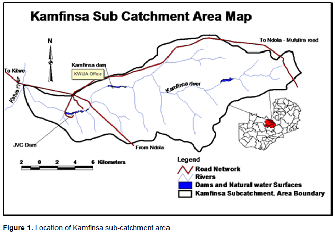
This study site is part of the Kamfinsa sub-catchment of the Kafue River watershed in Kitwe District of the Copperbelt Province of Zambia. It has annual rainfall varying from 1064 to 1302 mm per annum, and experiences three seasons namely: hot dry (September-November), rainy season (December-March) and the cold, dry season (April-August). The length of the growing season (LGS) is 157 days starting in the first ten days (dekad) of November and ceasing during the third dekad of March, and seasonal mean temperature of 21°C. According to Koeppen Classification, the climate is warm temperate with dry winters and hot summers (Cwa) and falling under dry sub humid with aridity index of 0.64 (Figure 1).

The vegetation of the study site is dominated by Miombo woodland, which characterizes most extensive tropical seasonal woodland and dry forest formations in Africa. Miombo is a vernacular word that has been adopted by ecologists to describe those woodlands dominated by trees of the genera Brachystegia, Julbernardia, and Isoberlinia Leguminosae, subfamily Caesalpinioideae (Campbell, 2007). The miombo region in Africa covers somewhere around 2.4 million km². Above-ground biomass stocking densities of the Miombo vary from 20 m³ ha-1 to as much as 150 m³. Characteristically, miombo is found in areas which receive more than 700 mm mean annual rainfall and where soils tend to be nutrient-poor (Campbell et al., 1996). Miombo woodlands cover substantial portions of southern Africa: Angola, Zimbabwe, Zambia, Malawi, Mozambique and Tanzania, and most of the southern part of the Democratic Republic of Congo. It is dominated by a few species, mostly from the genera Brachystegia, Julbernardia and Isoberlinia. Miombo is so-named after the Swahili word for a Brachystegia species. In the entire Miombo eco-region, Zambia has the highest diversity of trees and is the centre for endemism for Brachystegia tree species (Kalaba et al., 2013).
The Catchment starts from the source of Kamfinsa Stream in Sakania area of Ndola rural district, bordering Democratic Republic of Congo (DRC). Kamfinsa Stream drains the catchment with its five main tributaries, namely Chibwe, Mwambonalimo, Kafibale, Kamishishi and Kamatete streams (Figure 1). Kamfinsa Stream flows into Kafue River at a confluence about 200 m downstream from Kafue Bridge along the Ndola-Kitwe dual carriageway.
Sampling design
Sampling design for the landscape used GIS and remote sensing techniques to conduct land use mapping for the whole sub-catchment area as well as facilitate conducting of forest inventory. This approach allowed for analyzing the proxy variables for an ecosystem to measure the changes due to deforestation. The stratification was done for forest inventory based on vegetation types resulting from land use change. The data included tree diameters and height. Land cover change from the Miombo woodlands was also assessed using GIS and remote sensing.
Land cover change
The sets of data used for analysis were generated using GIS and remote sensing techniques based on Landsat forest cover and digital elevation models (DEM). They were used to estimate the forest cover change, soil erosion, and biodiversity change. The mapping Software tools were Envi 4.7, SAGA GIS and ArcGIS. Land use development over a period of 20 years was assessed from satellite images of the study site acquired for the years 1990, 2000 and 2010. The targeted images for landcover mapping were selected according to the time of year corresponding to the peak of vegetation greenness and, if possible, when cloud cover is low (Forestry Department, 2016). The images used in this study were for the period 1990, 2000, and 2010 corresponding to June and July.
The combination of Landsat's spatial resolution (30 x 30 m pixel size) with ability to detect electromagnetic radiation across the visible, infra-red and thermal wavelengths (Markham and Helder, 2012) has made it possible for the data collected by the sensor of high value to be used for classifying and mapping all manner of biophysical properties and alterations of these properties over time of the earth's surface (Roy et al., 2014). Landsat images consisting of spectral bands covering the study period were used for landcover analysis. The bands were used to create false colour composite images and subsequently used for production of the land-cover maps. The false colour satellite images were geometrically projected to UTM Coordinate System, datum WGS 84, zone 35s.
Considering that vegetation was a key component in the land cover mapping, false colour composite images were generated using 3 bands of Landsat namely, band 4 in near-infrared, band 5 in the mid infrared and band 2 in the visible part of the spectrum. Later, the false colour images were clipped using the Kamfinsa sub catchment area map boundary to generate the thumbnail images for each of the years 1990, 2000 and 2010.
The classification of thumbnail Landsat satellite images covering the sub-catchment area was done using ArcGIS 10 - spatial analyst extension. The classification method adopted was supervised classification using the Maximum Likelihood Classifier by visual interpretation followed by ground truthing. The land cover maps were digitally generated based on 6 classes of the IPCC (Fernández-Landa et al., 2016). Later, the land cover maps which were in raster format were converted to vector format. Statistics for each land cover class were generated.
Accuracy assessment
The accuracy of the land cover classification from supervised and unsupervised techniques are evaluated and presented as an error or confusion matrix table (Hasmadi, et al., 2009). In this study, to undertake the error assessment, the following steps were done (i) determine the total number of samples to be collected for each category, (ii) design an appropriate sampling scheme, (iii) obtain ground reference information at sample locations, (iv) produce error matrix and (v) evaluate the error matrices, producer accuracy, user accuracy, error of commission and error of omission.
The accuracy assessment was achieved by generating random points on the classified image and by performing Ground-truthing. To get accurate spatial data and classification result, the study also used Google Earth to collect feature type before ground-truthing. The aim of accuracy assessment was to quantitatively assess how effectively the pixels were sampled into the correct land cover classes (Rwanga and Ndambuki, 2017).
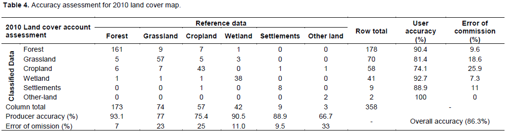
In assessing accuracy of the maps generated, a confusion matrix was used for the period under review. The result of the 2010 (Table 4 is correct for accuracy assessment) land cover map returned an overall accuracy of 86%, while 2000 was 81% and that of 1990 was 79%. Generally, all the land cover classes had better overall Kappa coefficient of 0.82.
Estimation of biomass and carbon stock
The study sites were stratified into homogeneous stands, for the purpose of the study, through visual interpretation of the georeferenced satellite imageries, google images of the site as well as the topographic map at a scale of 1: 50,000 and the vegetation map (1: 500,000 scale) for the Copperbelt Province produced by the Forestry Department helped to stratify the areas. Stratification was mainly into two, (i) mature undisturbed forest and (ii) the regrowth forest. The mature intact forest were parts of the forest that had not been severely affected by human activities, e.g., charcoal production, or clearing for agriculture purposes, while the regrowth stand was that, which had been recovering from human disturbances.
The sample plots were divided into three-nest circular sampling plots of 1 m, 10 m, and 20 m radius (Pearson et al., 2005). In total, 60 concentric sample plots of 0.126 ha were measured. The information recorded from each sample plot includes diameter at breast height (dbh) at 1.3 m above-ground surface, tree and shrub species names, and regeneration frequency. Smaller plots were used for regrowth because of the large density and diversity of species which makes the use of larger fixed plots time consuming (Syampungani et al., 2010). Tree volume (Tv) was calculated using the following formula:
where H is tree height, dbh is height at breast height (measured at 1.3 m from the ground) and 0.74 is a form factor.
Based on the Ndola Indigenous Sample Plots, noted that the best indicator of harvestable wood volume in natural forests was the Stand Basal Area (BA) and this was used to estimate the annual biomass annual increment of Miombo woodland. The two approaches for estimating the biomass of woody vegetation types are the volume method and the direct biomass estimation method. The volume method uses measured volume estimates that are then converted to dry biomass (ton ha-1) using a variety of tools (Forestry, 2016). The direct estimates of the biomass method use biomass allometric equations, as functions relating oven-dry biomass per tree as a function of a single or a combination of tree plant dimensions (Brown, 1997). The study used conversion factors as provided for in the IPCC best practices of 1996, which states that 47% of dry weight of total above-ground biomass is carbon and that below/above-ground ratio is 0.28 for tropical dry forests with above-ground biomass of 20 tons ha-1 (Kalaba et al., 2013).
In the case of estimating only annual biomass increase of wood in Miombo, a model by Endean (1967) was applied, which uses the basal area as a predictor variable. The basal area of a forest stand is found by adding the basal areas of all the trees in a field and dividing by the land area in which the trees were measured, and its unit expressed in m2 ha-1.
where biomass is above-ground wood mass (ton ha-1), and BA is basal area at breast height. Chidumayo (1990) estimated mean annual increment (MAI) in above-ground wood biomass in regenerating forest as 2.0±0.24 tons ha-1.
Estimation of soil erosion
Soil erosion is defined as the wearing-off of the land surface by physical forces such as rainfall, flowing water, the wind, ice, temperature change, gravity or other natural or anthropogenic agents. These agents abrade, detach, and remove soil or geological material from one point to be deposited elsewhere (Jones, 2007). Soil erosion is a process that occurs at all timescales; however, the natural rate is significantly increased through anthropogenic activity, and accelerated soil erosion becomes a process of degradation and thus an identifiable threat.
Land cover changes have been used to predict soil erosion which is related to ecosystem services both about water quality and future agricultural yield (Dale, 2007). Besides, soil erosion rates are largely a function of the proportion of bare ground (Dale, 2007). Remote sensing has been used to assess the length, area and density of the gullying system (Keay-Bright and Bright, 2006).
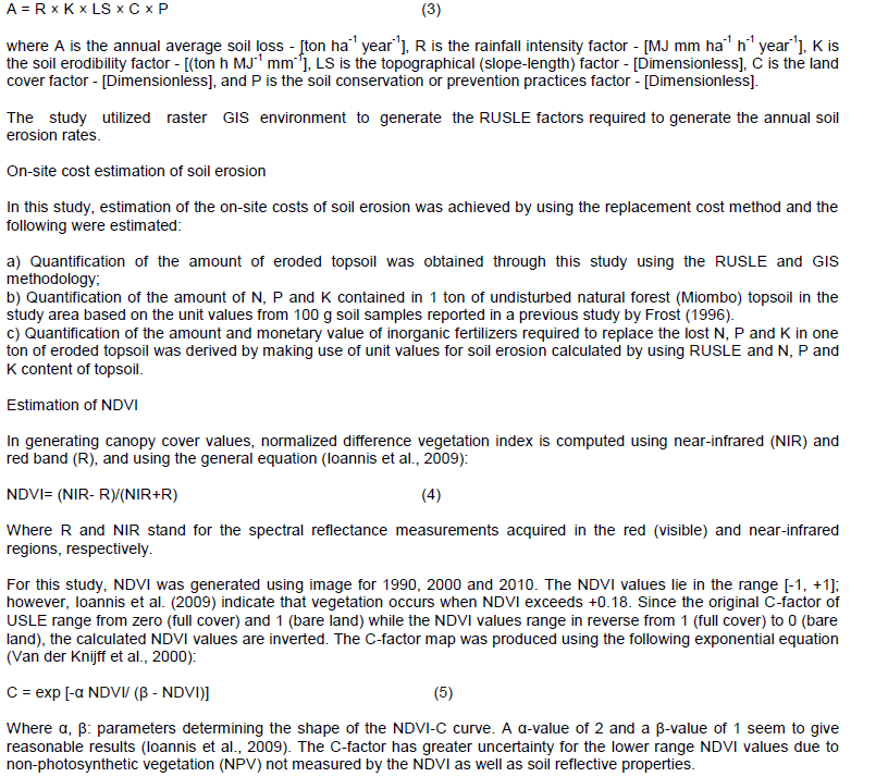
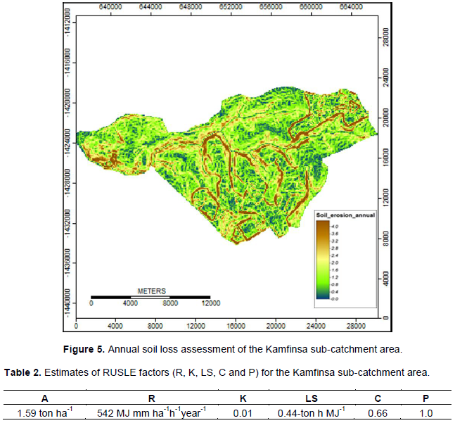
In the study, the raster layers corresponding to each of the six Revised Universal Soil Loss Equation (RUSLE) factors were created, stored, and analyzed with the ArcGIS and SAGA. The Soil Map was used to generate the K-factor, the rainfall data was used to generate the R-factor, the Landsat Images were used to generate the NDVI from which the C and P- factors were produced and finally the digital elevation model (DEM) was used to generate the L-factor and S-factor. This combination computed the estimated soil erosion potential for the entire study area. The RUSLE equation is widely used in predicting average annual soil loss based on soil erosion factors (Wischmeier and Smith, 1978; Renard et al., 1997) such as soil characteristics, topography, and land cover management. The RUSLE equation was used to estimate annual soil loss from the study area (Prasannakumar et al., 2012): Figure 5
Measuring changes in forest biodiversity
Estimation of land-use impacts on biodiversity, especially at a landscape scale is necessary to ensure systematic conservation planning (Desmet and Cowling, 2004). Vegetation indices can be used to represent environmental change. A broad range of contexts, including forest ecosystem destruction, degradation, and fragmentation (Holm et al., 2003), can be used in correlative studies to identify declines in ecosystem abundances (Carey et al., 2001) or species richness (Bar-Massada et al., 2012). Previously, the NDVI was used to generate maps, including the pioneering mapping of vegetation distribution and productivity in Africa (Tucker, 1985). Since then, there has been a number of studies in Africa, which include that of Martiny et al. (2010) who assessed the predictability of using NDVI in semi-arid African regions as well as the work of Higginbottom and Symeonakis (2014) who used the multi-temporal analysis of vegetation index data to show that NDVI and other vegetation indices can provide a sophisticated measure of ecosystem health and variation.
A study on spatial variability of species richness of birds in Kenya found a strong positive correlation between species richness and maximum average NDVI (Oindo et al., 2000). Different aspects of vegetation condition derived from vegetation indices such as NDVI contribute to the mapping of environmental variables which provide indications of species composition, abundance and distribution (Duno et al., 2007).
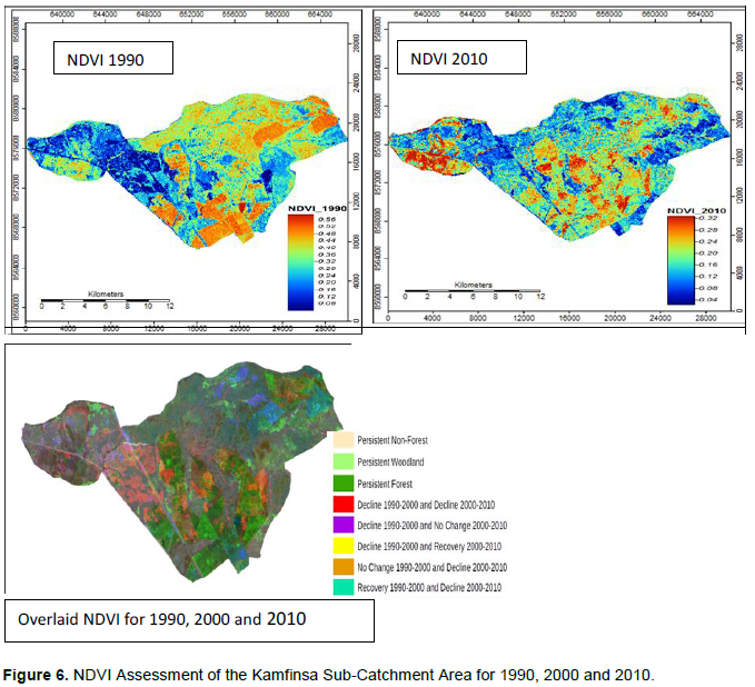
In this study, changes in forest biodiversity were measured by calculating the NDVI for 1990, 2000 and 2010. The NDVI for each time series was then overlaid in order to assess the changes that had occurred over the time period. The overlaid NDVI images using ArcGIS generated an image to assess the change and potential impacts on biodiversity. The image was used to evaluate the change in the vigor of plants by comparing the status in the undisturbed mature forest and the regrowth.
Overall estimation of the value of forests lost through deforestation
The valuation methods used in assessing the cost of deforestation on the ecosystem services were (i) Using the Replacement Cost method to assess the value of soil lost due to deforestation, which is an approach involving estimation of the expense of replacing an ecosystem service with a human-made product, infrastructure, or technology (Noel and Soussan, 2009) (ii) Assessing the value of forests (trees) in deforested areas using the economic value of biomass carbon. Recent forest valuation studies have used social cost of carbon emissions or the market value of carbon to assess the value of forests (Turpie et al., 2015) and (iii) by using NDVI to assess impact on forest biodiversity These vegetation indices can effectively be used to represent environmental change in a wide range of contexts, including habitat destruction, degradation and fragmentation (Holm et al., 2003) and can be used in correlative studies to identify declines in population abundances (Carey et al., 2001) or species richness (Bar-Massada, et al., 2012). These represent assessment of regulating, provisioning and supporting services, respectively.
White (1983) puts the figure for the "Zambezian phytochorollogical region" (of which miombo is the dominant element) at 3.8 million km2. Millington et al. (1994), based on remote sensing, suggested the more generally cited 2.7 million km2, but it is not exactly clear what they include in their estimate. Frost et al. (2003) suggest 2.4 million km2 for the miombo region, of which 466.000 km2 has been transformed. The miombo region is a mixture of woodland, degraded woodland and cropland.
Land cover change
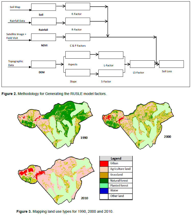
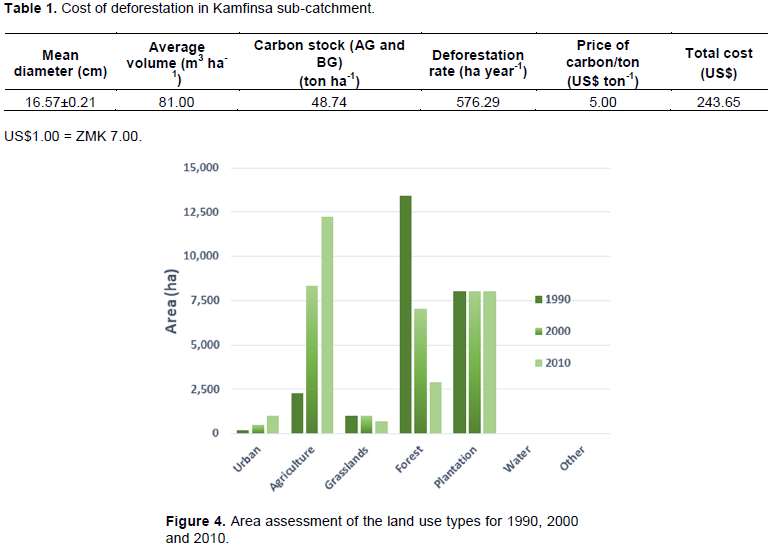
The land cover maps for 1990, 2000 and 2010 show that the natural forests ranged between 13,430 ha in 1990 to 7,081 ha in 2000 and only 2,904.7 ha in 2010. A total of 10,523 ha was lost in 20 years giving an average of 576.3 ha per year. On the other hand, agriculture land increased from 2,272 ha in 1990 to 8,333 ha in 2000 and 12,251 ha in 2010 (Figures 2 and 3). The tree plantations established for timber and poles remain the same during this period on 8,035 ha. Deforestation resulted in the loss of 10,525.80 ha (78.4%) of the forested area in Kamfinsa sub-catchment in 20 years. This deforestation is higher than the average rate of deforestation of the country, which was 300,000 ha per annum (0.60%), while the Copperbelt Province average was 0.84% (Forestry Department, 2016). This was a result of the Structural Adjustment Programme under which a lot of mine workers on the Copperbelt province, about 35,000 lost their jobs between 1991 and 2000 (Simutanyi, 2008). This resulted into unplanned settlement, high production of charcoal and increased land under agriculture as key drivers of deforestation since people had to seek for alternative livelihoods to survive. The primary cause of deforestation in the Kamfinsa sub-catchment area was agricultural activities resulting from new settlements due to job loss from the mines on the Copperbelt (Shitima, 2005).
Deforestation has led to changes of various ecosystem services including increase in soil erosion (Mumeka, 1986). Also, according to Shitima (2005), the forests in Mwekera provided other wood and non-wood forest products like charcoal, while Kalaba and Quinn (2013) indicated that the forests provided building poles, mushrooms, wild fruits, and roots which local communities traded to support their livelihoods. Besides, Kalaba et al. (2013) indicated that the vegetation composition of regrowth sites suggested that pre-disturbance land use affected the vegetation structure during recovery.
Biomass loss
The average biomass stocking density in Kamfinsa sub-catchment area of natural forests was 81 m3 ha-1 (Table 1 and Figure 4). This stocking density was equivalent to 38 tons of Carbon per hectare from above-ground biomass and 11 tons of Carbon per ha of below-ground biomass (based on IPCC suggested below/above-ground ratio which is 0.28 for tropical dry forests with above-ground biomass of 20 tons/ha). The above ground biomass results compare well with those generated by Kalaba et al. (2013) of 39.9 ton per hectare. Assuming a project-based price of Carbon at international market in 2015 of about US$5 per ton, the cost to the ecosystem of losing a hectare of forest was US$243.65. This cost, however, does not include other potential use of the forest, e.g., eco-tourism, as well as the actual cost of timber and non-wood forest products on the market. The cost would be much higher than that based on the sale of Carbon. According to Turpie et al. (2015), the world average price of carbon was between US$4 and US$8 per tonne. It was projected that carbon prices were to increase in future, possibly to as high as US$37–US$114 per tonne by 2050 (Chiabai et al., 2011). According to Turpie et al. (2015), the social cost of carbon was estimated to be US$29 per tonne and depending on location, Carbon stocks in Zambian forests are potentially worth about US$150 per ha (hectare) on average (once off) but range up to US$745 per ha for intact forests.
Soil erosion
The mean values calculated for using the Revised Universal Soil Loss Equation (RUSLE) were as follows; LS, the topographical (slope-length) factor was 0.44-ton h MJ-1 mm-1; K, the soil erodibility factor was 0.01-ton h MJ-1 mm-1; R, the rainfall intensity factor was 542 MJ mm ha−1 h−1 year−1; C, the landcover factor was 0.66, and the support practices assumed and hence given a uniform weight of 1. After all the RUSLE factors had been determined using GIS, they were combined in the GIS environment to come up with the soil erosion risk map of the area indicating different levels of soil erosion risk. The resulting map for the study shows soil loss values ranged between 0 and 16.78 ton ha-1 year-1 at the pixel level, with a mean value of 1.59 ton ha-1 year-1 (Table 2) with a standard deviation of 1.37. As observed, the average high annual soil loss occurred in areas with steep slopes and close to the stream banks as they were targets for cultivation. According to Turpie et al. (2015), the estimated average annual soil erosion in the Copperbelt area was 2 ton ha-1.
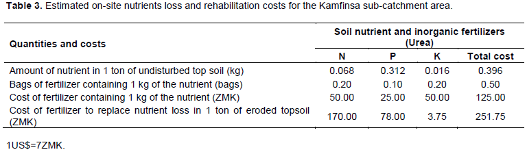
On-site soil erosion cost
The on-site cost due to nutrient loss from 1 ton of eroded soil is equal to the monetary value of specific inorganic fertilizers needed to replace the N, P and K contained in that ton of eroded soil. The replacement cost of nutrients in one ton of eroded topsoil regarding inorganic fertilizers was found to be Zambian Kwacha (ZMK) 251.75 (US$35.96) only for N, P, and K and does not include other nutrients and materials naturally found in topsoil. This amount, therefore, underestimates the actual cost of soil loss, including soil nutrient from one ton of eroded topsoil. The study (Table 3) estimated that 1 ton of soil loss cost ZMK 251.75 (US$35.96). The soil erosion risk assessment observed that 1.59 tons of soil was lost per hectare of land annually, and this meant that the total cost per hectare was at ZMK 400.28 (US$57.18). However, this may be an underestimation since the loss includes soil structure, soil biodiversity, soil organic matter, other soil matter minerals and organic matter.
According to Quamsah et al. (2000) and Amegashie et al. (2012), while it was useful to know the magnitude of soil nutrient losses, their on-site costs were equally important. The increased area under cultivation from 2,272 ha in 1990 to 12,251 ha in 2010 increased the exposure of the land to soil erosion. Cultivated fields did not show specific conservation practices. The area converted to agriculture was mainly from the natural forests. According to Shawa (2012), Mwekera Dam (within the Kamfinsa sub-catchment area) was affected due to soil erosion resulting in siltation in the stream and
the dam which is the only water source for the National Aquaculture Research Development Centre (NARDC) and the Zambia Forestry College (ZFC). Shawa (2012) further observed that the dam was shallower due to siltation; hence it affected the water flow and fish production, especially during the dry season.
Change in biodiversity
It has been recognized that there is a relationship between species richness and primary productivity in terrestrial ecosystems (Waide et al., 1999). Net primary productivity (NPP) of forests as well as species richness increase towards the equator and that vascular plant richness correlates with NPP; hence these results are consistent with recent meta-analyses showing that the relationships between productivity and species richness of both plants and animals in natural ecosystems are predominantly positive (Gillman et al., 2014). Vegetation indices can be used to represent an environmental change in a wide range of contexts. This change includes habitat destruction, degradation, and fragmentation (Holm et al., 2003) and can be used in correlative studies to identify declines in population abundances (Carey et al., 2001) or species richness (Bar-Massada et al., 2012). The NDVI for 1990 and 2010 show differences regarding minimum and maximum values. In 1990, the maximum was 0.56, while that of 2010 shows 0.32. It means that the forests in 1990 were denser as compared to the forests in 2010. In fact, as may be noted, the forest in 1990 had 13,431 ha of natural forest which declined to only 2,901 ha in 2010 threatening and reducing the potential existence of different species of fauna and flora. The plantations according to the map remained at 8,035 ha. Areas of continuous agricultural activities remain persistent non-forests. The water body reduced from 11.50 ha in 1990 to about 6.30 ha in 2010 and further reduced the habitat for water-based fauna and flora.

The NDVI images analyzed for 1990, 2000, 2010 indicated that the maximum vegetation composition was negatively affected and reduced from 0.56 in 1990 to 0.32 in 2010 (Figure 6). Therefore, when there is a reduced NDVI, it generally means primary productivity is affected negatively and hence that the quality of forest reduced over time in terms of biodiversity and habitat. Areas of continuous agricultural activities remain persistent non-forests, and this means that there were no activities related to agroforestry to replace the lost trees. A study on spatial variability of species richness of birds in Kenya found a strong positive correlation between species richness and maximum average NDVI (Oindo et al., 2000). Different aspects of vegetation condition derived from vegetation indices such as NDVI contribute to the mapping of environmental variables which provide indications of species composition, abundance, and distribution (Duno et al., 2007).
According to CBD (2001), in the absence of biodiversity, there would be no ecosystems and no ecosystem functioning. Also, there is evidence that productive complex forest ecosystems are less diverse under the same conditions and more resilient than less productive ones (Ozanne et al., 2003). Highly prone to catastrophes are forests that comprise relatively few species and provide relatively few goods and services. The loss of biodiversity means the loss not only of the habitat of different species found in the area but also the loss of livelihoods of the people living in and around these forests.