Full Length Research Paper

ABSTRACT
This study analyzed latent heat flux from Amazon deforestation runoff above the Central/North American Boundary currents from 1988-2015. The purpose is to propose Atlantic hurricane intensification from the heat flux via condensation. The author divided those currents into ten areas of evaporation considering water budget data and regional and water-vapor-transport. A spreadsheet program consisting of two models had three inputs. Evaporation in each of the ten areas became the first input. For simplicity, each area’s evaporation decremented incoming runoff one time, and passed through less runoff, considering the currents’ average velocities and ocean condensation residency. Recent high-flow runoff data, limited from June 1 through November 30, a typical hurricane season, became the other inputs: all Amazon runoff (Model-A), only Amazon deforestation runoff (Model-O). The spreadsheet converted the condensation heat flux from each season (km3) into 10^17 J/day. This study compared those values to the 10^17 J/day wind energy of Category-1 or Category-3 hurricanes, finding order of magnitude similarity for such a crude comparison. The author then correlated hurricane Emily’s July 2005 daily path interface with the daily latent heat flux from the deforestation runoff. The analysis indicated that daily heat flux interfacing with Emily’s path measured 5.82% of a Category-3’s 10^17 J/day. When considering reuse runoff in deforested areas aggregate from 1970 to 2004, that 5.82% increases to possibly 12.85%. This study’s simple analysis is by like terms (J/day) and similar order of magnitude (10^17) only, necessitating a more complex analysis.
Key words: Deforestation, hurricanes, latent heat flux, modelling, runoff.
INTRODUCTION
Recent estimates illustrate the historic costs and potential energy of Atlantic hurricanes. In 2005, Hurricane Katrina cost $161 billion (NOAAFastFacts, 2013). In 2012, Sandy caused $18.75 billion in insured property losses alone (Artemis, 2013) and $65 billion in total cost. In 2005 Emily became the earliest-forming Category-5 hurricane on record for the month of July in the Atlantic basin (Franklin and Brown, 2006). Considering the prevention of human and dollar costs, a study indicates Rapid Intensification (RI) of hurricanes is notoriously difficult to predict and can contribute to severe destruction and loss of life (Balaguru et al., 2018). Studies have categorized the intensity of these hurricanes by their maximum wind speed. A Category-1 rating requires a one-minute- average maximum sustained winds at 10 m above the surface of 33-42 m/s, a Category-3 requires 50-50 m/s (Saffir and Simpson, 1973).
Several model simulations demonstrated the Amazon runoff’s Rapid Intensification (RI) of North Atlantic hurricanes. One earlier study (Vizy and Cook, 2010) using atmospheric models identified how the Amazon River plume’s presence increases the stability of the Barrier Layer (BL) near the surface water. This allowed warm Sea Surface Temperature (SST) anomalies to increase the number of tropical storms reaching hurricane strength by 61%. A later study (Balaguru et al., 2012), illustrated the relationship between SST increase from the BL formed by Amazon River discharge region and more accurately simulated the tropical Atlantic atmosphere. Recently, another study (Gouveia et al., 2019) proposed a conceptual model showing the influence of Amazon runoff increase and its impact on the SST. That model indicated warming of the amazon plume, thereby influencing latent flux heat to the tropical Atlantic atmosphere. However, these SST studies are limited in that they find no quantified anthropogenic cause for the RI of Atlantic hurricanes. This study drills down to one specific and significant anthropogenic cause for RI– Amazon deforestation runoff. Figure 1 summarizes this study.
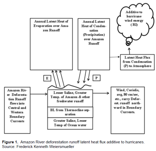
The comparisons herein are by like terms and similar order of magnitude only, noting that Emanuel, (1998) indicates large quantities of latent heat flux are necessary to perform work on the air. Nonetheless, this study attempts to quantify the deforestation runoff latent heat flux missing from the literature. Regarding that Amazon deforestation runoff, a source reports almost all precipitation over deforested rainforest (e.g. Amazon) is lost as runoff (Raven and Berg, 2006). That is due in large part to the impervious nature of the upper plinthic soil in the Amazon rainforest. Two Amazon rain forest studies reported this: northern Para, Brazil (Chaves et al., 2008) and in southern Rondonia, Brazil (de Moraes et al., 2006). After that Amazon deforestation runoff flows into its discharge plume it becomes part of the North Brazil Current, the first of the boundary currents analyzed here. The aim of this study is to calculate the actual latent heat flux volumes from that deforestation runoff in the Central/North American Boundary currents. In addition, this study shows when and where those heat flux volumes may have intersected a recent hurricane’s path. It also converts those volumes into hurricane wind- energy terms to see what percentage they are of a typical hurricane’s wind-energy. It does that considering the whole of the Central/North American Boundary currents as well as the individual currents. In this way, the author hopes to show the mechanisms linking Amazon River deforestation runoff to the Rapid Intensification (RI) of Central/North American Boundary current hurricanes.
METHODOLOGY
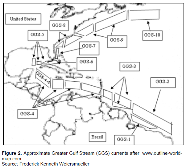
This study utilizes an Excel spreadsheet program, using MS Office Version 14.0.7015.1000. Henceforth it will refer to the spreadsheet program simply as “Spreadsheet”. Latent Heat of Condensation Potential Energy (LHCPE) refers to flux from Model-A Amazon runoff and from Model-O Amazon runoff. The author refers to the ten main divisions of the Central/North American Boundary currents in Figure 2, as the Greater Gulf Stream (GGS). The GGS includes the Amazon discharge plume (GGS-1), North Brazil (GGS-2), Guiana (GGS-3), Caribbean Sea (GGS-4), Loop (GGS-5), Florida (GGS-6 & GGS-7) currents. The GGS also includes the northern part of the traditional Gulf Stream (GGS-8, GGS-9, and GGS-10). Some GGS-n are divided into geometric GGS-n-n subdivisions. The Mariano (2016) website maps indicate these currents with curvy arrows of one-degree longitude/latitude (MarianoArrowData, 2013). This study approximates the distance between these arrows as 100 km, latitude or longitude (WikipediaLongitude, 2019). The author estimates 162 traversal days for a hypothetical runoff floater in GGS-1 to reach the GGS-10 endpoint, based on 11,200 km approximate distance northward, at a typical GGS velocity of 80 cm/sec (Mariano, 2016). Dividing each GGS geometric surface areas by the known global ocean surface area, 361.9 × 10^6 km2 (Eakins and Sharman, 2010), yields a ratio, the Surface Area Coefficient (SAC). The SAC factor assists in calculating the annual evaporation over each GGS current. Supplementary Materials Item A, (SMA), details the SAC geometric factor calculations for all ten GGS currents. This study assumes 7 days residence for evaporation over oceans and 8.9 days over land after (van der Ent and Tuinenburg, 2017).
Spreadsheet section A – Factors and GGS evaporation
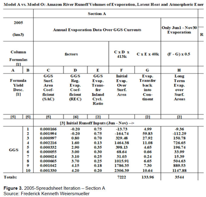
The SAC factor provides a good point to introduce the Spreadsheet, which has a matrix with three sections: Section A (factors and GGS evaporation), Section B (Model-A) and Section C (Model-O). That matrix is the source for most of the tables, figures, and SMa herein. Figure 3 illustrates Section A of the 2005 Spreadsheet iteration. The Section A values are constant for all the 1988-2015 Spreadsheet iterations. The SAC factor in column C becomes a variable in the columns F and G formulas. Additionally, two other latitudinal factors effect calculations of evaporation. First, this study developed the Regional Evaporation Coefficient (REC) factor by the author’s interpolation. after Wunsch (2005) Figure-3-Right. That figure details the Northern hemisphere atmospheric residual heat flux in Petawatts (PW), see SMB. This provided a basis for the Regional Evaporation Coefficient (REC) factors in column D of Figure 3. The REC factor becomes a variable in the column F formula. Second, this study developed the Evaporation Transfer Inland Cycling Ratio by the author’s interpolation after van der Ent and Savenije (2013) , see SMC. This provides the basis for that ratio in Column E Figure 3, which accounts for water vapor transport inland variations. The latitudinal variance data in that study only covered the period 1990–2009. However, another study (de Moraes et al., 2006) using the Earth system model GFDL-ESM2G, indicates only a 3% increase in the Ocean to Land Water Vapor Transport between the end of the 20th century (1999) and the end of the 21st century (2099). That is only 0.18% increase for the six years data, 2010-2015, missing in van der Ent and Savenije, 2013) study. Therefore, the author used van der Ent and Savenije (2013) latitudinal ratios for the REC factor over the complete 1988-2015 timeframe. The ratio becomes a variable in column G formula. Columns F and G formulas also utilize the water budget data factors (Trenberth et al., 2007), that is, Ocean Evaporation of 413/year and Ocean Evaporation Transfer Inland of 40k km3/year. Also, Model-A and Model-O utilize the factor of Ocean Precipitation of 373k km3/year (Trenberth et al., 2007).
Spreadsheet sections B and C – Model-A and Model-O
Figure 4 illustrates the 2005 Spreadsheet iteration for column H of Section A, and all of Section B, and Section C. The Spreadsheet contains several bracketed numbers “[n]” that help pinpoint certain cells, columns, or rows. Note [1] refers to the Column Formulas row and the Formula Yield Descriptions row. Note [2] refers to Evaporation Transfers Inland Cycling Ratios for each current. Note [3] indicates Initial Runoff (Jun - Nov) input into the discharge plume for both Model-A and Model-O. Note [3] also refers to the runoff leaving each successive GGS current. Note [4] refers to the first type of Spreadsheet proportional expression, “L x Mprev/Iprev”; that is, Model-O-Evaporation equals Model-A-Evaporation times the ratio of Model-O runoff to Model-A runoff; Note [5] refers to GGS current numbering and SAC factor. Note [6] refers to REC factor for all GGS-n currents. Note [7] refers to the second type of Spreadsheet proportional expression containing the ratio of condensation-to-evaporation 373k/413k (Trenberth et al., 2007) in Sections B and C; and [7] also refers to the phenomenon – when ocean water vapor condenses (precipitation) the latent heat releases to the surrounding atmosphere, and the water molecules return to the ocean (Lindsey, 2009; Met, 2021). This leaves some lessor evaporative flux residue. The Spreadsheet column-labels I through O, have asterisk suffixes. Like-numbered asterisks indicate a similar IF-THEN-ELSE formula logic, not displayed in the Column Formula row. For example, column-labels “I*” and “M*”, Equation 1 and 2 respectively, prevent circular reference and division by zero. They involve columns Q and R as memory cells off the main worksheet, not shown in Figure 4. Thus, any GGS-n zero-result in Sections B and C is expressed by a four-digit decimal number, “0.0001”. That number indicates exhaustion of a GGS-n’s runoff by evaporation; and it prevents circular reference and division by zero.

=IF(Q22<=0,0.0001,SUM(I21-H22)) (1)
=IF(R22<=0,0.0001,SUM(M21-L22)) (2)
The column labels with two, three and four asterisks have more- involved IF-THEN-ELSE logic. Their purpose is the correct accounting of evaporative/condensation values once runoff exhaustion occurs in the previous GGS-n current and results in a value of “0.0001”.
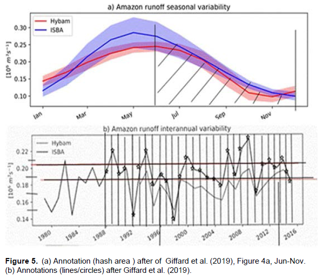
The calculation of Model-A Initial Runoff Input in Figure 4 is 2555 km3, column I. To arrive at that initial input volume, the author has annotated lines onto Figure 5a and 5b after Giffard P, et al. (2019).
Calculation of Amazon Model-A Initial Runoff (Jun-Nov).
First, Figure 5a indicates the Amazon flow-rate varies during the year. The author annotated parallel lines onto Figure 5a, for the June 1 through November 30 seasonal Amazon runoff (Goldstein, 2021). The author approximated that hashed-area as 45% of the ISBA annual runoff. The Giffard et al. (2019) study employed two data sets: ISBA satellite measurements and HYBAM Obidos-station gauge measurements. In Figure 5b, the interannual measurements of the HYBAM data (1993-2015) partially correlated to ISBA data (1970-2015). The Giffard et al. (2019) study reported that where the years overlapped in the two data sources, the HYBAM data corresponded. Also, the ISBA data correlated well with the 1988-2019 annual deforestation data from another study (INPE, 2019) for Model-O calculations. Therefore, this study used the ISBA-CTRIP data to calculate the Initial Runoff (Jun - Nov) values. Interestingly, the Amazon runoff flow is almost three times greater during the rainy season (0.275 × 10^6 m^3/s, May-Jun) than during the dry season (0.10 × 10^6 m^3/s, Dec-Jan). Second, Figure 5b indicates Amazon runoff flow-rate varies interannually. In Figure 5b, the author has annotated vertical/horizontal lines and small circles to interpolate the Amazon runoff interannual data. For the 2005 interpolation, the author converted the values to10^12 m3/year, using the 31.54 × 10^6 s per year SI units conversion factor. This yields 5677 km3 for Jan-Dec, and after applying the 45% factor, yields 2555 km3 runoff. That becomes the Spreadsheet 2005 Model-A “Initial Input Runoff (Jun - Nov):” in column I, that is, runoff received by GGS-1. The Spreadsheet accounted for this calculation regarding the other 1988-2015 iterations in the same manner.
Calculation of Amazon Initial Model-O deforestation runoff (Jun-Nov)
Turning to Section C, the Model-O Initial Runoff Input is 4.13 km3 in column M of Figure 4. For that data, the author utilized the annual deforestation satellite data (INPE, 2019), (PRODES Amazon, 2020). For 2005, those sources indicate yearly deforestation area of 19,014 km2 or 19.0 × 10^9 m2 (INPE, 2019). To calculate the deforestation runoff, this study utilized a factor from another study (Bruno et al., 2006) - Amazon rainforest has 0.53 m3 water holding capacity per m3 of soil, nearly uniform with soil depth. Therefore, taking conservatively the upper one meter of soil from Bruno (2006), then 0.53 m3 of water per m2 of soil exists over the 19.0 x 10^9 m2 of deforested soil. That yields 10.07 × 10^9 m3 water or 10.07 km3. Therefore, as in Model-A, applying the 45% factor (Giffard et al., 2019) yields 4.53 km3 for the June through November 2005 deforested runoff input, up to this point.
However, the author considered two smaller factors that restrict that 4.53 km3 Model-O yield, namely the exoreic evaporation and groundwater losses. Model-A accounted for these two factors in its Obidos station data. The Amazon Basin contains 6.3 × 10^6 km2 (Goulding et al., 2003), a fraction of the 149 × 10^6 km2 global land area, that is, glaciers, habitable land, beaches, dunes, exposed rocks, salt flats, deserts (Ritchie and Rose, 2019), or 4.2%. Also, a World Water Resources monogram finds 2100 km3/year direct global groundwater runoff to the ocean and 1100 km3/year global exoreic evaporation (Shiklomanov, 1998). Applying the 4.2% factor yields 88.2 km3 of groundwater exited directly to ocean and 46.2 km3 of exoreic evaporation occurred from the Amazon Basin. In addition, the Amazon Basin totaling 6.3 × 10^6 km2 (Goulding et al., 2003) received 19,014 km2 (INPE, 2019) deforestation in 2005, or 0.3%. This study established earlier that deforested land returns most precipitation to runoff (Chaves et al., 2008), (de Moraes et al., 2006). Therefore, after applying the 0.3% factor, the yields are 0.14 km3 of exoreic evaporation and 0.26 km3 of groundwater direct to ocean from the Amazon Basin 2005 deforested area. Thus, 4.53 km3 minus 0.14 km3 exoreic minus 0.26 km3 groundwater yields 4.13 km3, the 2005 Model-O “Initial Input Runoff (Jun - Nov):” in column M, received by GGS-1. The Spreadsheet accounted for this calculation regarding the other 1988-2015 iterations, see SME for details.
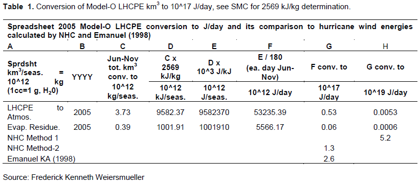
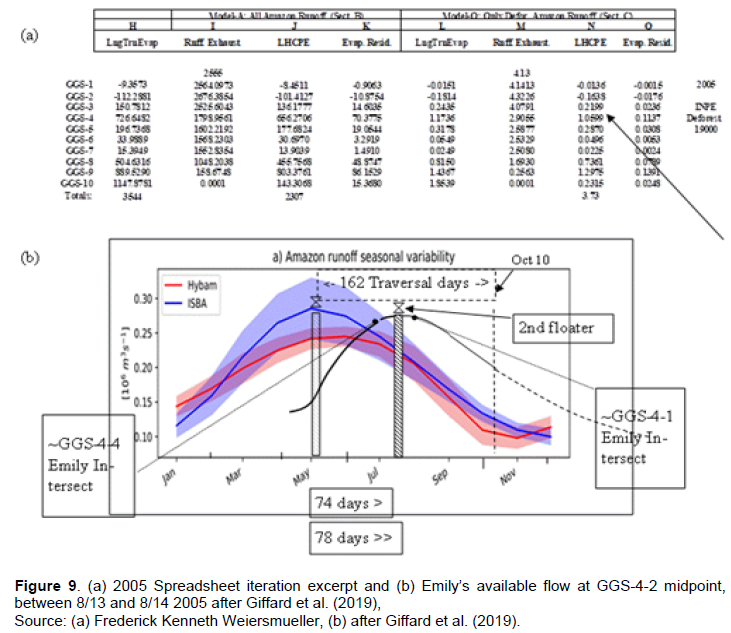
Conversion of Model-O LHCPE km3 to 10^17 J/day in Table 1.
The 2005 Spreadsheet iteration calculated 3.73 km3 Model-O- GGS-LHCPE at the bottom of column N in Figure 4, cumulative from the GGS-n components. Table 1 details the Spreadsheet conversion of 2005 LHCPE from seasonal km3 into 10^17 J/day. This study maintains that atmospheric potential energy, LHCPE, resides in the atmosphere ahead of the path of the hurricane. And it maintains the LHCPE is additive, intensifying existing hurricane wind energy causing category changes through condensation in the hurricane’s concentric outer rain-bands. This study compares that LHCPE potential energy to studies of hurricane wind energy from two other studies. Those are: the NHC Method-2 study of wind energy (NHC, 2020; Emanuel, 1998) for Category-1, and the non-NHC study (Emanuel, 1998) for Category-3. Those two studies calculate the daily wind energy by integrating the hurricane dissipation that occurs mostly in the atmospheric surface layer area covered by a circularly symmetric hurricane.
The NHC Method-1 (NHC, 2020; Gray, 1981) for an average hurricane or Category-1 was not considered for this study. The NHC Method-1 calculated total energy released through the volumetric cloud/rain formation, from the eyewall to the outer radius of a hurricane. There are any number of concentric rain-bands that radiate out from the eyewall, interspersed with non-rainbands (Zehnder, 2020). Another study (de Moraes et al., 2006) using radar reflectivity data, found that the distant rainbands contain the deep convective cores and they typically mature or die by the time they reach the inner core. Therefore, this study assumes LHCPE added its potential heat energy to the atmosphere earlier in the outermost rain-bands, before they spiral inward. For completeness, Table 1 lists the much larger NHC Method-1 calculation.
RESULTS
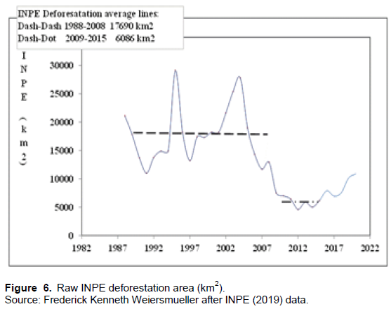
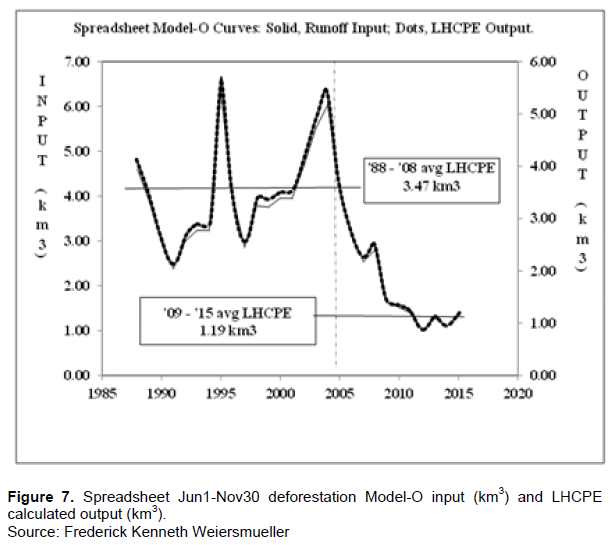
The author considered Table 1 2005 demonstration a crude comparison, nevertheless finding order of magnitude similarity in regards to hurricane RI, and will attempt to refine the comparison here. Henceforth, unless otherwise specified, “LHCPE” refers to the Model-O-LHCPE in the “Totals:” Spreadsheet row, calculated from Jun-Nov deforestation runoff. Figure 6 graphs the INPE (km2) raw deforestation data from 1988-2015 before the Bruno (2006) factor, 0.53 m3/m2, and the Giffard et al. (2019) factor, 45% of annual, are applied. Two averages illustrate significant differences in Figure 6: the raw 1988-2008 INPE average of 17,690 km2 versus the 2009-2015 INPE average of 6,086 km2. It is interesting to note that the raw deforestation data for 2016-2020 has begun an upswing: 7,900, 6900, 7500, 10,100 and 10,900 km2, respectively (INPE, 2019). The average for this five-year upsurge is 8660 km2. That is 30% more than the 2009-2015 low average of 6086 km2. Figure 7 graphs the Spreadsheet LHCPE (km3) output from the Jun-Nov INPE deforestation runoff input to the 1988-2015 Spreadsheet iterations. SME lists the 1988-2015 Spreadsheet iteration results in more detail. The 19,014 km2 raw data from 2005 was converted to 4.13 km3 input to the Spreadsheet. That resulted in 3.73 km3 of Jun-Nov LHCPE. Figure 7 echoes the 1988-2008 versus the 2009-2015 difference in LHCPE averages seen in Figure 6 in terms of seasonal INPE averages. Noteworthy, is a high mark 29,100 km2 in 1995, which resulted in 5.71 km3 of seasonal LHCPE. It compares to the low mark of 4600 km2 in 2012, which resulted in only 0.90 km3 of seasonal LHCPE. Next, this study looked at Hurricane Emily’s 2005 path through any specific GGS-n(-n) areas and its wind speeds along that path.
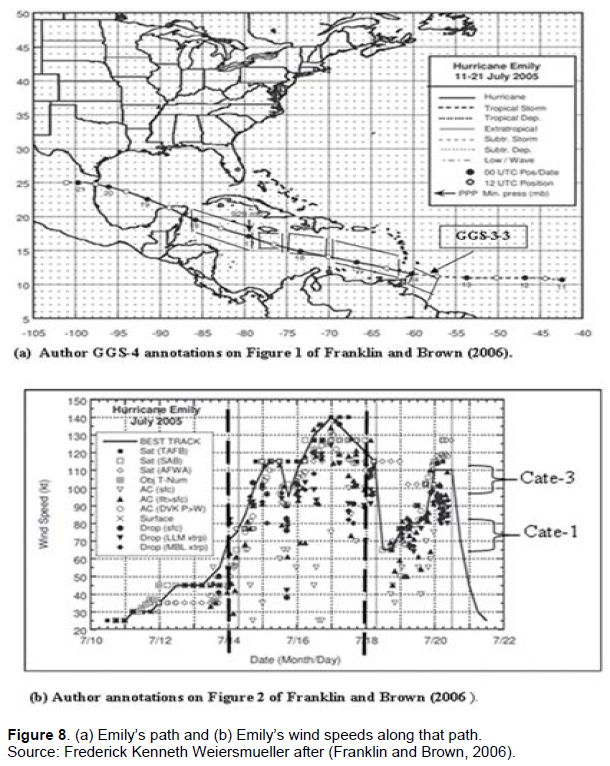
Hurricane Emily’s path and wind speed through GGS-4 in 2005
Figure 8 contains the best track and wind speeds of Emily with annotations after (Franklin and Brown, 2006). The report indicates Hurricane Emily formed at roughly 0112 UTC 14 July approximately 85 n mi east-southeast of Grenada (very eastern end of GGS-4-1). The author’s annotations on Figure 8a, illustrate that Emily traversed the entire GGS-4 area The author’s annotations on Figure 8b illustrate Emily’s wind speed during that time. Emily was a Category-3 or greater during approximately 87% of the time from 0112 UTC 14 July through 0000 UTC 18 July. RI to Emily would have occurred during that timeframe from LHCPE or other factors such as SST. Furthermore, an NHC report states Emily’s winds peaked to Category-4 early on 7/15/2005 and Emily briefly became a Category-5 as well 0000 UTC 17 July about 100 n mi to the southwest of Jamaica (Franklin and Brown, 2006). Therefore, this study will conservatively consider Emily as at least Category-3 for the entire GGS-4 area, during the four days, 7/14/2055 0000 UTC until 7/18/2005 0000 UTC. This study then analyzed the 2005 seasonal LHCPE attributed to GGS-4 during Emily’s path from GGS-4-1 to GGS-4-4.
Seasonal LHCPE and maximum runoff flow during Emily’s path through GGS-4
The arrow in Figure 9a points to the 1.06 km3 Model-O-LHCPE that accumulated in GGS-4 during the hurricane season. Emily’s path took it through the entire GGS-4, always maintaining Category-3 and above. That 1.06 km3 LHCPE from GGS-4 is 28.4% of the 2005 seasonal 3.73 km3 LHCPE calculated in column N. That significant seasonal LHCPE could have contributed to Emily’s RI. In Figure 9b, this study looked at the heavy May-June runoff flow after Giffard et al. (2019). That is in relation to the typical GGS-n(-n) considering the typical 80 cm/sec Amazon runoff flow. Figure 9b illustrates that heavy May-Jun runoff flow interfacing Emily’s path from 8/14-8/18 in 2005. Figure 9b depicts a hypothetical runoff floater, “X”, on May 1 at the start of GGS-1, the discharge plume. The second hypothetical runoff floater marks Emily’s 4-day intersection with that May-June runoff flow. SMF indicates roughly 30 days of Amazon runoff flow within GGS-4. That allows four 7-day evaporation cycles, as per van der Ent and Tuinenburg (2017) to preset GGS-4 with significant LHCPE. Figure 9b also indicates the heavy flow at the approximate start of GGS-4-1 and it continues to the end of GGS-4-4 in Emily’s timeframe, considering where the curve would be in each case. It is an important point that GGS-4 receives in mid-July through mid-October that heavier deforestation runoff flow from May through August as reported by Giffard et al. (2019). That runoff flow is approximately 0.27 m3s-1. That is 2.7 times the Dec-Apr flow of 0.10 m3s-1 and again indicates possible RI from deforestation runoff. These heavy runoff volumes in Figure 9 occurring in Hurricane Emily’s path, carried high percentages of the seasonal LHCPE km3 and add weight to the argument that they contributed to Emily’s RI. Interestingly, that LHCPE (km3) from deforestation runoff possibly contributes RI during each hurricane season. It varies only as Amazon deforestation varies. Whereas, other RI phenomenon such as Atlantic Multidecadal Oscillation – Seas Surface Temperature (AMO-SST) and El Niño–Southern Oscillation (ENSO) Wind-Shear, may not be available for RI in each hurricane season.
DISCUSSION
SME summarizes all the 1988-2015 Spreadsheet iterations of Model-O output. It also summarizes all that output converted into 10^17 J/day as demonstrated in Table 1 for just the 2005 iteration. Figure 10 graphs those 1988-2015 Spreadsheet iterations of LHCPE converted to seasonal 10^17 J/day and their associated INPE. The years 1995, 2003, 2004 and 2005 are notable in Figure 10 for their high annual deforestation (km2) and corresponding high LHCPE and 10^17 J/day. However, the question remains whether any of that 0.53 x 10^17 J/day from Jun-Nov 2005-LHCPE intersected with the path of Emily in 2005 and did it cause intensification. Here this study will determine that. Table 2 is a special demonstration of the 2005, Table 1 calculations The Results section analyzed the “seasonal” LHCPE (km3) of GGS-n(-n) which carried the max-runoff volumes that hurricane Emily could have utilized as RI. Here, this study breaks down that seasonal volume into “daily” contribution of LHCPE (10^17 J/day) towards RI of Emily in its Category-3 formation. Then LHCPE (10^17 J/day as a percentage of Category-3 hurricane wind energy in 10^17 J/day is calculated for each GGS-n(-n) in the path of the hurricane.
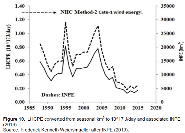
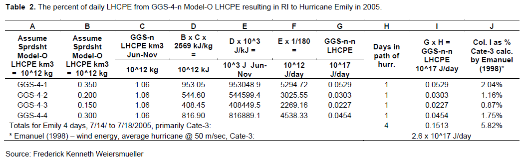
The Table 2 special iterations of Table 1 indicate LHCPE could have possibly contributed 5.82% of the 10^17 J/day towards Emily as a Category-3 hurricane in GGS-4.
However, so far the author had only considered 2005 INPE “fresh” deforestation – 19014 km2 for 2005 - and had not included the additional 113710 km2 from pasture reuse of deforested area from 1970 to 2004 (INPE, 2019). That totals instead 132724 (see SMG) for greater input to Model-O in 2005. Applying that increased deforested area to the Spreadsheet calculations (see SMD, SME, and SMG) yields 2.34 km3 of Model-O LHCPE output at GGS-4 instead of 1.6 km3. As a result, the special iteration of Table-1 in SMD indicates the LHCPE could have possibly contributed 12.85% towards Emily as a Category-3 hurricane in GGS-4, and more indication of possible RI.
A disparity may appear in that the 2.34 km3 Model-O LHCPE in GGS-4 is only 0.35% of the 656.27 km3 Model-A LHCPE in GGS-4 for 2005. The following analogy should clarify that. In this analogy, the 2.34 km3 contributes 12.85% to the areal formation (Emanuel, 1998) of a Category-3 hurricane from a Category-2 hurricane. The 656.27 km3 contributes 18% (see SMH for analogous calculation), to the volumetric formation (NHC, 2020) of a Category-1 hurricane from a tropical storm. The Category-1 volumetric formation from a tropical storm requires 5.2 x 10^19 J/day, whereas the Category-3 areal formation from a Category-2 requires a smaller 2.6 x 10^17 J/day.
In addition, the author notes this study conservatively applied the first meter down in Methodology regarding the 0.53 m3/m2 rate (consistent down to 10 meters) of deforested runoff after Bruno RD, et al.( 2006). If deforestation drained soil water at 0.53 m3/m2 five meters down instead, then the Spreadsheet calculations would indicate even more RI. This study possibly represents the first time in the literature that hurricane RI analysis was tailored to the Amazon high runoff in the flooding season and its intersection with the hurricane season, Jun-Nov.
Other coexisting RI phenomenon
Studies have found other factors in the formation of these hurricanes. For example, an NHC report indicated Hurricane Denis had made portions of the Caribbean Sea warmer and hence more favorable for the development of hurricane Emily (Franklin, 2005).
However, this presentation calculates anthropologic LHCPE from deforestation as a possible RI factor. That LHCPE-RI may act alone or it may coexist with phases of other RI phenomenon that are intermittent. Proper treatment of other RI that are intermittent. or stand-alone phenomenon coexisting with LHCPE-RI requires another study.
CONCLUSION
This study advances the oceanographic and marine science state of knowledge in the following ways. This study quantifies evaporation from Amazon deforestation runoff over the Central/ North American Boundary currents (GGS) and its latent heat flux from condensation (LHCPE). This study utilized only six months of annual Amazon basin river runoff data (Giffard et al., 2019) and annual deforestation data (INPE, 2019). That June 1 through November 30 data is appropriate to a typical hurricane season (Goldstein, 2021). That demarcates the deforestation latent heat flux properly as a cause for RI. This study looked at a substantial timeframe of data, 1988-2015, twenty-eight years regarding that LHCPE. This study analyzed 2005 Hurricane Emily’s RI from its path-interface with the Latent Heat of Condensation Potential Energy (LHCPE) from deforestation runoff to be significant in orders of magnitude. That RI could be additive or stand-alone regarding other RI phenomenon. The comparisons herein are by like terms and similar order of magnitude only. Emanuel (1998) indicates large quantities of latent heat flux are necessary to perform work on the air. Nonetheless, this study repeatedly points to Amazon deforestation runoff’s difficult-to-assess role in RI. What exact proportion exists between the LHCPE quantified here and its RI (hurricane kinetic energy product) remains unsolved. A more complex mathematical analysis is necessary. This study’s findings suggest future experiments. The first suggestion is a study quantifying stable oxygen-18 isotopes originating from Amazon deforestation-site runoff insertion, present in ocean hurricane atmosphere, via reconnaissance aircraft such as the Global Hawk drone. It is known that the stable oxygen isotopes differ in seawater versus in river water (Craig and Gordon, 1965). A reconnaissance aircraft study of that type could be definitive in assessing deforestation runoff percentages in hurricane atmospheres. The second suggestion relates to the calculation here of deforestation runoff as a factor in Meridional Overturning Circulation (MOC) slow down studies (Feng et al., 2014; Bryan, 1986; Rahmstorf, 2003). The precipitation that is resultant from deforestation runoff LHCPE (Lindsey, 2009) remains in the North Atlantic Ocean at the end of GGS-10. Would that additional volume of warmer water influence the tipping point towards Meridional Overturning Circulation Slow Down?
CONFLICT OF INTERESTS
The author has not declared any conflict of interests and is sole creator of this document.
REFERENCES
|
Artemis (2013). Artemis Catastrophe bonds, insurance linked securities, reinsurance capital & investment, risk transfer intelligence. |
|
|
Balaguru K, Flotz GR, Leung LR (2018). Increasing Magnitude of Hurricane Rapid Intensi?cation in the Central and Eastern Tropical Atlantic. Geophysical Research Letters. |
|
|
Balaguru K, Chang P, Saravanan R, Jang CJ (2012). The barrier layer of the Atlantic warmpool: formation mechanism and influence on the mean climate. Tellus A: Dynamic Meteorology and Oceanography, 64(1):18162. |
|
|
Bruno RD, da Rocha HR, de Freitas HC, Goulden ML, Miller SD (2006). Soil moisture dynamics in an eastern Amazonian tropical forest. Hydrological Processes 20(12):2477-2489. |
|
|
Bryan FO (1986). High-latitude salinity effects and interhemispheric thermohaline circulations. Nature 323:301-304. |
|
|
Chaves J. Neil N, Germer S, Neto SG, Krusche A, Elsenbeer H (2008). Land management impacts on runoff sources in small Amazon watersheds. Hydrological Processes 22(12):1766-1775. |
|
|
Craig H, Gordon LI (1965). Deuterium and Oxygen 18 variations in the ocean and the marine atmosphere. Spoleto, Italy, Pisa, Consiglio nazionale delle richerche, Laboratorio de geologia nucleare. |
|
|
de Moraes JM, Schuler AE, Dunne T, Figueiredo RDO, Victoria RL (2006).Water storage and runoff processes in plinthic soils under forest and pasture in eastern Amazonia. Hydrological Processes 20(12):2509-2526. |
|
|
Eakins BW, Sharman GF (2010). Volumes of the World's Oceans from ETOPO1. |
|
|
Emanuel KA (1998). The power of a hurricane: An example of reckless driving on the information superhighway. Massachusetts Institute of Technology - Kerry Emauel Professor of Atmospheric Science (website). |
|
|
Feng QY, Viebahn JP, Dijkstra HA (2014). Deep ocean early warning signals of an Atlantic MOC collapse. Geophysical Research Letters 41(16):6008-6014. |
|
|
Findell KL Keys PW, van der Ent RJ, Lintner BR, Berg A, Krasting JP (2019). Rising Temperatures Increase Importance of Oceanic Evaporation as a Source for Continental Precipitation. Journal of Climate 32(22):7713-7726. |
|
|
Franklin J(2005). Emily Discussion 8, National Hurricane Center, Miami, FL. |
|
|
Franklin JL, Brown DP (2006). Tropical Cyclone Synoptic Report-Hurricane Emily, National Hurricane Center, Miami FL. |
|
|
Giffard P, Llovel W, Decharm B (2019). Contribution of the Amazon River Discharge to Regional Sea Level in the Tropical Atlantic Ocean. Water 11(2348):16. |
|
|
Goldstein Z (2021). Atlantic & Eastern Pacific Climatology. National Hurricane Center Miami Fl. |
|
|
Goulding M, Barthem RB, Ferreura EJG (2003). The Smithsonian Atlas of the Amazon. Smithsonian Institute Press, Washington, DC. ISBN 10:1588341356 and ISBN 13: 9781588341358. |
|
|
Gouveia NA, Gheradi DFM, Aragao LEOC (2019). The Role of the Amazon River Plume on the Intensification of the Hydrological Cycle. Geophysical Research Letters 46(21). |
|
|
Gray W (1981). Further analysis of tropical cyclone characteristics from rawinsonde compositing techniques. Monterey(CA): Naval Environmental Prediction Research Facility (U.S.). |
|
|
Hence DA, Houze RA (2012). Vertical Structure of Tropical Cyclone Rainbands as seen by the TRMM. Journal of the Atmospheric Sciences pp. 2644-2661. |
|
|
HurricaneHuntersAssoc (NHC) (2020). How much Energy does a Hurricane Produce? |
|
|
Instituto Nacional de Pesquisas Espaciais (INPE) (2019). National Institute for Space Research (Instituto Nacional de Pesquisas Espaciais INPE) p/o PRODES (Deforestation) Accumlated Deforestation Rates per Year in the Legal Amazon States, orig. 1985). |
|
|
Lindsey R (2009). Climate and Earth's Energy Budget. |
|
|
Mariano A (2016). Surface Currents in the Atlantic Ocean. |
|
|
MarianoArrowData (2016). Ocean Surface Currents, Data. |
|
|
Met (2021). How does the tropical cyclone obtain its energy? UK Meter.Serv. |
|
|
NOAAFastFacts (2013). Coastal Fast Facts, s.l.: Office of Coastal Management. |
|
|
PRODES Amazon (2020). Earth Observation INPE. |
|
|
Rahmstorf S(2003). The Current Climate. Nature 421:699. |
|
|
Raven PH, Berg LR (2006). Environment. John Wiley and Sons, NJ. ISBN: 10:0471704385 and ISBN 13: 9780471704386. |
|
|
Ritchie H, Rose M (2019). Land Use. |
|
|
Rogers RR, Yau MK(1989). A Short Course in Cloud Physics. Vol: 113, 3rd ed. Oxford and New York, Pergamon Press. ISBN: 0-7506-3215-1. |
|
|
Saffir H, Simpson R (1973). Saffir-Simpson Hurricane Scale. |
|
|
Shiklomanov IA(1998). Water Resources: A New Appraisal and Assessment for the 21st Century, UNESCO. |
|
|
Trenberth KE, Smith L, Qian T, Dai A, Fasulo J (2007). Estimates of Global Water Budget and Its Annual Cycle Using Observational and Model Data. Journal of Hydrometeorolgy 8(4):758-769. |
|
|
Tuinenburg OA, Hutjes RWA, Kaba P (2012). The fate of evaporated water from the Ganges basin. Journal of Geophysical Research 117(D1). |
|
|
van der Ent RJ, Savenije HHG (2013). Oceanic Sources for Continental Precipitation. Water Resources Research 49(7):3993-4004. |
|
|
van der Ent RJ & Tuinenburg OA (2017). The residence time of water in the atmosphere revisited. Hydrology and Earth System Sciences 21(2):779-790. |
|
|
Vizy EK, Cook KH (2010). Influence of the Amazon/Orinoco Plume on the summertime Atlantic climate. Journal of Geophysical Research 115(D21112):1-18. |
|
|
WikipediaLongitude (2019). Length of a degree of longitude. |
|
|
Wunsch C (2005). The Total Meridional Heat Flux and Its Oceanic and Atmospheric Partition. Journal of Climate 18(21):4374-4380. |
|
|
Zehnder JA (2020). Anatomy of A Cyclone, |
|
Copyright © 2024 Author(s) retain the copyright of this article.
This article is published under the terms of the Creative Commons Attribution License 4.0


