Vegetation has a marked effect on runoff and soil moisture and plays an important the hydrologic cycle. The Watershed Resources Management (WRM) model, a process-based, continuous, distributed parameter simulation model developed for hydrologic and soil erosion studies at the watershed scale lack a crop growth component. As such, this model assumes a constant parameter values for vegetation and hydraulic parameters throughout the duration of hydrologic simulation. A crop growth algorithm based on the original plant growth model used in the Environmental Policy Integrated Climate (EPIC) model was developed for coupling to the WRM model. The developed model was tested for yield simulations using data from a field plot within the Oyun River basin, Ilorin, Nigeria. Model prediction closely matched observed values with R2 of 0.9 for the years under study. This model will be incorporated into the WRM model in other to improve its representation of vegetation growth stages in a natural basin. This modification will further enhance its capability for accurate hydrologic and crop growth studies.
Change in the vegetation of a watershed alter the natural hydrologic cycle and significantly affects runoff (Cao et al., 2009). Vegetation, which was once thought to only play a relatively minor role and was ignored or treated as a static component in hydrologic models has now been recognized as one of the most important factors affecting the hydrologic cycle (Chen et al., 2014). The pivotal role that vegetation plays in the global water balance cannot be neglected. The interactions between ecosystems and water resources are important for studying the effects of environmental management (land-use change) on hydrologic processes, and thus to provide solution to problems of water resources and watershed management. Vegetation is an important component of terrestrial ecosystem and must be considered in integrated models for simulating hydrologic processes (Strauch and Volk, 2013). Thus, the need to fully represent soil water – crop growth dynamics in hydrologic models for accurate representation of biophysical and hydrologic processes cannot be overemphasized. Crop growth modeling concepts evolved in the 1960s with the major aim of understanding the fundamental biological processes of single crops (van Ittersum et al., 2003).
Crop modeling started in the United States with the development of the Environmental Policy Integrated Climate (EPIC) model in the 1980s to simulate the impacts of soil erosion on soil productivity. Over the years, the EPIC model has evolved into a comprehensive agro-ecosystem model that includes major soil and water processes related to crop growth and environmental effects of farming activities (Wang et al., 2006). Its crop growth component offers major advantage in that it contains a single model with the capability of simulating multiple crop growth and development in any region of the world. Several agro-ecosystem models such as Water Erosion Prediction Project (WEPP) model (Flanagan et al., 1995), Soil and Water Resources Tool (SWAT) model (Arnold et al., 1998), Agricultural Land Management Alternative with Numerical Assessment Criteria (ALMANAC) model, Wind Erosion Predictions System (WEPS) model, etc have either simplified or modified the EPIC’s crop growth model and incorporated it to suit their different research objectives. Nowadays, crop growth models are not only used to predict crop yield or study crop physiological processes but also part of many hydrologic models and agricultural decision support tools (Multsch et al., 2011).
A realistic representation of a hydrologic system is important for water resources development and management at the watershed scale (Kiniry et al., 2008). In most hydrologic models, crop parameters such as hydraulic roughness are kept constant throughout a period/season of hydrologic simulation resulting to a gross oversimplification of reality and inaccurate models results (Pauwels et al., 2007). The Watershed Resources Management (WRM) model (Mbajiorgu, 1995a) is a process-based, continuous, distributed-parameter hydrologic model. As a continuous simulation model, WRM model requires a crop growth component in other to simulate effect of crop growth on hydrologic processes. Currently, this model lack such capability as it assumes constant parameter values for vegetation and land cover management throughout duration of simulation. Therefore, it is imperative to implement a crop growth module in WRM in other to enhance the model capability to realistically simulate hydrologic processes. The objective of this study is to develop a crop growth subroutine that is compatible with the WRM model structure. The model was further applied to simulate corn yield for a location in Nigeria.
The crop model follows the general concept described in the EPIC model and consists of a single modeling approach for simulating multiple crops by changing input parameter values. Crop phenological development is based on daily accumulated heat units, harvest index is used for partitioning yield, Monteith’s approach for potential biomass accumulation, and actual biomass actual biomass accumulation obtained by determined using Leibig’s Law of the Minimum by considering water and temperature stress factors. The crop growth model is capable of simulating annual and perennial crops. Annual crops grow from planting date to harvest date or until accumulated heat units equal potential heat units for the crop while perennial crops maintain their root systems throughout the season.
Crop phenological development
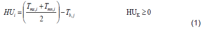
The model use thermal time is represented by heat units (HU) or also commonly referred to as growing degree-days (GDD) for modeling crop phenological development. Arnold et al. (1998) stated this as:
Where, HUi = value of heat unit on day I; Tmx,i = daily maximum temperature (°C); Tmn,i = daily minimum temperature (°C); Tb,j =crop specific-based temperature of crop J (no growth occurs at or below Tb).
Crop phenological development is generally seen as a heat unit index ranging from 0 at planting to 1 at physiological maturity of a crop. This is calculated as:
Where, HUIi = heat unit index for day i; HUk = sum of daily heat units from planting date to current date; PHUj = potential heat units required for crop j to grow to maturity.
Crop potential growth
Potential daily biomass accumulation is based on radiation-use efficiency (RUE) using interception of photosynthetic active radiation by crop canopy (as represented by the leaf area index and light extinction coefficients) and an energy to biomass conversion factor (Ascough II et al., 2014). RUE represents the above ground biomass production per unit of light intercepted by the crop canopy. A conversion factor of 0.45 or 0.43 can be easily used to convert incident total solar radiation to photosynthetic active radiation (PAR) above the plant canopy (Kiniry et al., 2008). These authors defined PAR as the definitive band of wavelengths pertinent to photosynthetic response which is inherent in the RUE approach. PAR interception by crop canopy is modeled using Beer’s Law (Monsi and Saeki, 1953):
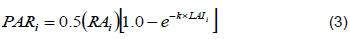
Where, PARi = intercepted photosynthetic active radiation on day i (MJ/m2/d); RAi = solar radiation on day i (MJ/m2/d); 0.5 = factor for converting solar radiation to PAR; k = extinction coefficient; LAIi = leaf area index on day i. Accurate value of PAR is very important in crop modeling as it drives photosynthesis and potential biomass simulation. PAR simulation in several ecohydrologic models (SWAT, EPIC, WEPP, etc) assumes a constant (0.65) for light extinction coefficient (k), while the ALMANAC model uses different values of k for different crop species and for different row spacing (Kiniry et al., 1992). Also, Equation 3 shows that PAR is calculated using 50% of daily total solar radiation. However, Kiniry et al. (2008) pointed out that only 2% or less of the energy in the PAR waveband is utilized by crops during photosynthesis and biomass production. These authors developed a function to accurately determine the extinction coefficient of PAR (kPAR) from the extinction coefficient of total solar radiation (ks) as stated below.

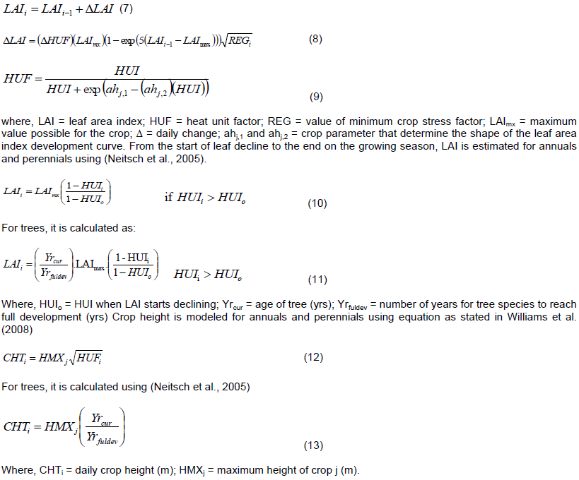
Crop cover and height
Leaf area index (LAI) is the leaf area per unit ground area irrespective of leaf orientation (Wilson, 2011). Accurate simulation of crop light interception, transpiration and dry matter/biomass accumulation depends on the accurate estimation of LAI (Birch et al., 1998). The leaf area development model uses a sigmoid function to represent pre-senescence growth of LAI, while power function is used to represent a decline in leaf area index during post-senescence period (Nair et al., 2012). LAI is simulated as a function of heat units, crop stress and crop developmental stages. From emergence to start of leaf decline, LAI is calculated as:
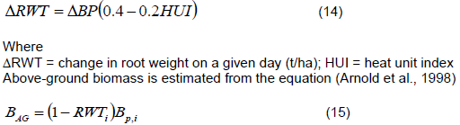
Root development
Biomass partitioning to roots is calculated when the fraction of daily biomass partitioned to roots changes linearly from 0.4 at emergence to 0.2 at maturity based on phenological stages, with the remainder going to the canopy (Ascough II et al., 2014). These authors calculated daily change in root weight as:
Rooting depth normally increases from the seeding depth to a crop-specific maximum which is usually attained before the crop phenological maturity (Neitsch et al., 2005). It is calculated as a function of heat units and potential root zone depth and is stated as:
Crop yield
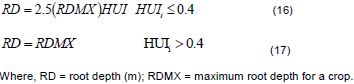
Crop yields are mostly reproductive organ removed from the field during harvest. Harvest index is the fraction of the above-ground dry biomass removed as dry economic yield (Neitsch et al., 2005). These authors noted that this index varies from 0.0 – 1.0. The harvest index (HI) concept stated in Williams et al. (2008) was adopted for modeling crop yield. This concept was employed in the EPIC model, SWAT model and so many other models. It is obtained by multiplying harvest index with above-ground biomass.
Crop water use
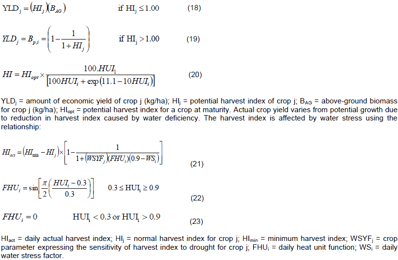
Water is the major limiting factor for crop growth. Water uptake by crop roots is driven by transpiration and depends on the moisture content of the soil. In this model, root grows to a crop-specific maximum and water compensation is possible when part of the root is in dry soil layers (van Ittersum et al., 2003). The potential water use is estimated using the leaf-area-index relationship (William et al., 2008):
Where, up = water use; Ep = potential water use; Eo = potential evaporation; LAI = leaf area index; Ë„ = water use distribution parameter; Z = soil depth; RZ = root zone depth; UC = water deficit compensation factor.
Crop growth stress factors
Crop growth is limited by water, temperature, nutrients and aeration stresses. Only water and temperature stress factors were considered in this study. Lack of water limits biomass production and also affects transpiration. The water stress factor (REG) is computed considering the water supply and water demand (William et al., 2008):
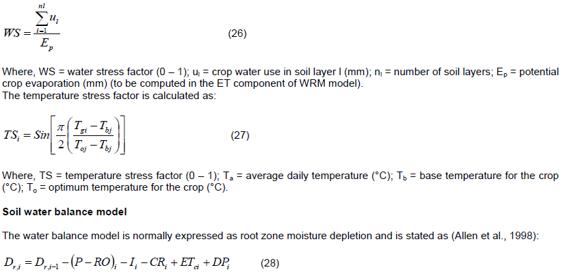
Where, Dr,i = root zone depletion at the end of day i (mm); Dr,i-1 = water content in the root zone at the end of the previous day, i-1 (mm); ROi = runoff from the soil surface on day i (mm); Ii = net irrigation depth on day i that infiltrates the soil (mm); CRi = capillary rise from the groundwater table on day i (mm); ETci = crop evapotranspiration on day i (mm); DPi = water loss out of the root zone by deep percolation on day i (mm). Van Ittersum et al. (2003) reported that the major approaches for modeling soil water balance is either by the tipping bucket approach or the Richards approach. The tipping water bucket was adopted for this study because it is straightforward, used to calculate water available to crops for long time periods and has been used in many crop models.
Watershed resources management (WRM) model: Theory
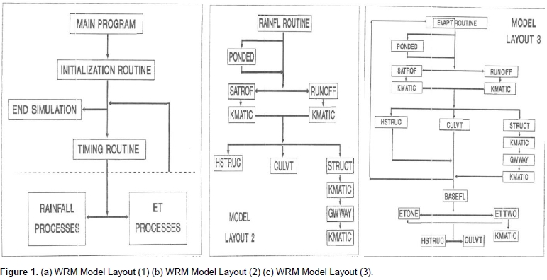
The hydrologic processes as incorporated in the WRM model are modeled by finite differences of the mass, momentum and energy conservation equations. WRM model is applicable at the basin scale, in planning, forecasting and operational hydrology; in design flow estimation, to the study of environmental impacts of land use changes, and to soil and water conservation planning (Mbajiogu, 1995b). Empirical equations, derived from relating physical quantities experimentally and validated independently, are also employed for the development of WRM model. The specific fundamental process equations, and equations used to track the physical state of the system are presented for each of the component program modules as follows: initialization routine; timing routine, rainfall-event routine, ponded-infiltration routine, runoff routine, saturation-runoff routine, kinematic-flow routine, conservation-structures (terraces) routine, culvert routine, evapotranspiration-event routine, base flow routine, soil-moisture accounting and subsurface-lateral flow routines (Mbajiorgu, 1995a).
The spatial structure of the European Hydrological System (SHE) model was adopted for distribution of hydrologic responses and parameter specification. A comprehensive, rigorous and state-of-the-art theory of the hydrologic processes as employed in the WRM model is found in Mbajiorgu (1992). Mathematical representations of hydrologic and soil erosion processes employed by WRM model to represent a hydrologic system are canopy interception storage, evapotranspiration, infiltration, saturated subsurface flow, overland and channel, reservoir routing, soil erosion and sediment routing, channel-flow transport, terrace-channel flow, grass-waterway flow and culvert flow. The general layout of the WRM model computer program in terms of its module is as shown in Figure 1(a), (b) and (c) (Mbajiogu, 1995a).
The main subprogram is essentially a specification and overall control module. It calls five subroutines, namely: initialization, timing, rainfall event, evapotranspiration event, and an optional report generator. These subroutines as a group are termed 1st Order routines. Other subroutines called directly from them are grouped together as 2nd Order routines, which in turn call 3rd order routines. Operation of WRM model components and its synthesis is fully described in Mbajiorgu (1992, 1995a). The crop model has a modular structure by design and is compatible with the WRM model framework making it easy to be incorporated into the WRM main program as a subroutine. The default crop parameters were determined based on values from William et al. (2008) and was adopted to develop a crop parameter database for this model.
Model evaluation
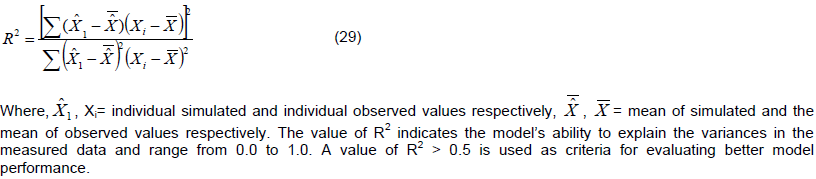
Model performance was evaluated using the linear regression coefficient of determination (R2) which is calculated as:
Crop model development
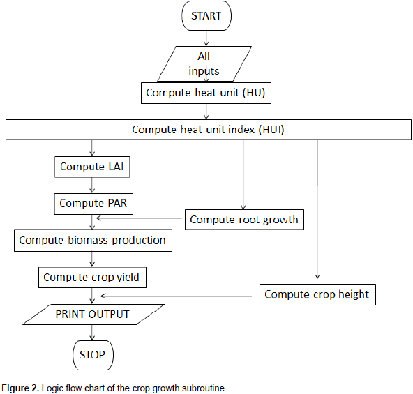
Figure 2 show the logic flowchart of the crop growth subroutine which simulates crop growth, canopy interception of solar radiation, conversion of intercepted PAR to biomass, division of biomass into roots, above ground biomass and economic yield and root growth. Crop development is driven by temperature with growth duration dependent on degree days. Every crop species has a unique base and optimum temperatures which is used to obtain its heat unit index. Daily changes in biomass production are observed when crop available water at the root zone is insufficient to satisfy potential evapotranspiration. Yield is simulated as a fraction of the total aboveground dry matter at maturity.

The crop model is modular in design and was developed with C# programming with a Microsoft Visual Studio-based graphical user interface (GUI). It consists of the above-mentioned crop growth processes and a Microsoft Excel file for crop growth parameters. The model’s GUI makes it easier for users to select inputs (climate, crop, soil characteristics), perform simulations and view results. Simulation starts with the initialization of model parameters and reading of input data from external files. The model during run time implements daily calculations for all growth process equations till crop physiological maturity is attained. The graphical user interface (GUI) has a friendly interface which allows user to create a project/open existing project, select crop type with parameters and perform simulation. Model results are displayed and can be viewed using Microsoft Excel.
Model application
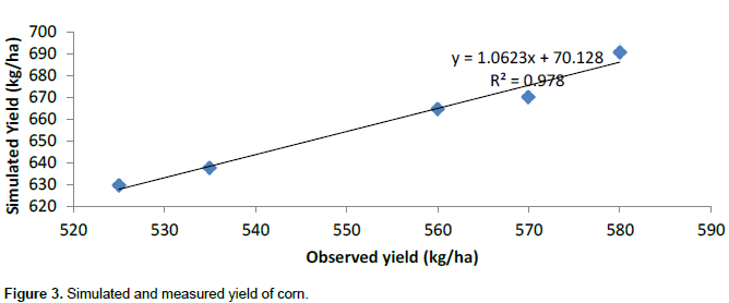
The model was tested with corn yield data from a farmland located within Oyun River Basin, Ilorin, Kwara State, Nigeria to evaluate the model capability for crop yield simulation. This basin is largely used for farming and lies within the grass plains of Nigeria. It has an average elevation of 251 m and lies between Latitude 9°50´ and 8°24´N and Longitude 4°38´ and 4°03´E. The area experiences rainy season from April to October, having a mean annual rainfall of 1700 mm and mean monthly maximum and minimum temperature of 31 and 29°C respectively.
Model input
Weather data of daily rainfall, maximum and minimum temperature, solar radiation, wind speed and relative humidity were obtained from the Meteorological Station of the National Centre for Agricultural Mechanization (NCAM), Ilorin, Kwara State, Nigeria. Crop specific inputs for corn were obtained from William et al. (2008) and used to perform model runs. Potential heat unit for corn was calculated from planting to maturity and used as input for yield simulation. The water balance was simulated using the FAO Penman Monteith method. Seasonal corn yield data for 2004 to 2008 were obtained from the National Centre for Agricultural Mechanization (NCAM), Ilorin and used for comparison with simulated yields. Difference between observed and simulated yields for corn is presented in Figure 3. The choice of crop was dependent on continuous yield data availability for the study.