Full Length Research Paper
ABSTRACT
Garlic is the major bulb crop next to onion in Ethiopia. Lack of stable and high yielding cultivars is one of the major problems for production and productivity of garlic in the country. Identification of adaptable, stable and high yielding genotypes under varying environmental conditions prior to release as a cultivar is the first steps for plant breeding. Therefore, developing high yielding and stable varieties is the primary objective of garlic improvement in this country. Nine garlic genotypes were evaluated to study their adaptability and stability in eight environments of Tigray region, northern Ethiopia. The experiment was carried out in randomized complete block design with three replications in four locations over two years. In this study, additive main effects and multiplicative interaction (AMMI) and genotype by environment interaction (GGE) biplot analyses were used in the evaluation of test environments and genotypes. The AMMI analysis showed that the effects of genotype, environment and genotype × environment interactions were significant (P<0.01) on bulb yield. AMMI evaluation confirmed that the three main components accounted for 89.8% of the whole genotype by environment interaction. The which-won-where view of the GGE biplot showed that environments used for this study grouped in to two mega-environments, with two different winning genotypes G9 and G7. Both AMMI and GGE biplot analysis identified promising genotypes. Genotype G9 (Bora-1/16) had the highest average yield performance and stability compared to other cultivars and should be used in breeding programs for new garlic variety development.
Key words: Additive main effects and multiplicative interaction (AMMI), bulb yield, garlic, genotype by environment interaction (GGE) biplot, stability analysis.
INTRODUCTION
Garlic (Allium sativum L.), is from the genus Allium and family Alliaceae grown as edible bulbous crop in the world. It is originated in Central Asia (Brewster, 1994). It is a diploid with the basic chromosome number of 2n=16 oldest cultivated vegetable and second most extensively species of obligated apomixes, therefore its reproduction system is vegetative through its cloves. Garlic is the produced Allium next to onion (Batth et al., 2013; Diriba, 2016; Dejen, 2018). It is used for seasoning in many ingredients as well as for medicinal and spiritual purposes (Tewodros et al., 2014). It is extensively cultivated throughout the world including Ethiopia. In Ethiopia, 15381.01 ha of land have been underneath of garlic cultivation with a production of about 1386643.07 tones (CSA, 2017).
Garlic is the most widely cultivated bulbous crop in Ethiopia and it has a wide range of climatic and soil adaptation. However, its production and productivity are very low due to many biotic and abiotic bottlenecks such as lack of high yielding varieties, non-availability of quality seeds, imbalanced fertilizer use, lack of irrigation facilities, lack of appropriate disease and insect pest management and other agronomic practices, low storability, and lack of appropriate marketing services (Getachew and Asfaw, 2010; Mohammed et al., 2014). Therefore, multi environment variety trials (MET) on different crops including garlic are essential, because of the existence of genotype × environment (GE) interactions (Gauch and Zobel, 1997). The development of high yielding varieties with wide adaptability is the basic target of plant breeders. Genotype by environment interaction evaluation is important for genotype selection and cultivar recommendation, and to identify appropriate production and test environments (Singh et al., 2016; Habte et al., 2019; Ngailo et al., 2019). Bulb yield and days to maturity of garlic is disposed to environmental changes resulting in variable yield due to the significant effect of genotype-by-environment interaction (Tewodros et al., 2014).
Assessment of different genotypes across locations and over years is now not only essential to select and recommended high-yielding cultivars but also to identify suitable areas that represent the ideal environment (Yan et al., 2001). Moreover, the efficiently developed high-yielding new cultivar must have a stable overall performance and broad adaptation over a wide range of environments. A genotype is considered as stable if it has adaptability for a trait of economic significance throughout diverse environments. The environmental factor (E) usually represents the biggest issue in analyses of variance, however, it is not applicable to cultivar selection; only G and GE are relevant to significant cultivar comparison and ought to be viewed simultaneously for making selections (Yan and Kang, 2003). As there are no studies on G x E in garlic crop in Ethiopia particularly in Tigray regional state, the importance of conducting such studies throughout principal garlic producing locations have been suggested. Genotype x location (GL) interaction effects are of special interest for breeding programmes to identify adaptable, stable and high yielding genotypes and test locations. Additive main effects and multiplicative interaction (AMMI) analysis and genotype plus genotype by environment interaction (GGE) biplot analysis were widely used a multivariate technique for interaction investigation (Gauch et al., 2008; Mohammadi et al., 2010). AMMI biplot evaluation is regarded to be a high quality tool to diagnose GEI patterns graphically. AMMI analysis can also be used to find out the stability of the genotypes across locations using the (principal component axis (PCA) scores and AMMI stability value (ASV). Purchase (1997) developed the AMMI stability value primarily based on the AMMI model’s principal components axis 1 and 2 scores for each cultivar, respectively.
Another powerful statistical model GGE biplot model combines the two principal effects, that is, genotypes (G) plus the G × E interaction (GE). This method is proven to be beneficial to decide which-won-where pattern of the multi-locational trials facts thereby figuring out high-yielding and stable cultivars and the power to discriminate and become aware of representative test environments (Yan, 2001). Now-a-days, it is a common practice through crop breeders to use GGE models in explaining G × E interaction and analyzing the overall performance of genotypes and test environments (Yan et al., 2007; Ngailo et al., 2019). GGE biplot, especially, is useful, to graphically represent the GE interaction, and to rank the studied genotypes and environments (Ngailo et al., 2019). According to the GGE biplot, a highly stable genotype would have a shorter projection on to the average environment coordinate (AEC) abscissa, irrespective of its direction (Yan and Kang, 2003). These two statistical analyses (AMMI and GGE) have broader relevance for agricultural researchers because they pertain to any two way data matrices, and such data emerge from many kinds of experiments (Gauch, 2006). In Ethiopia, there is no ample information on the genotype by environment interaction effects on bulb yield and yield related traits of garlic. Therefore, the objective of this study were: to assess the stability and yield performance of garlic genotypes over years and across locations; and to identify stable and high yielding candidate genotype(s) for possible release.
MATERIALS AND METHODS
Study sites and planting materials
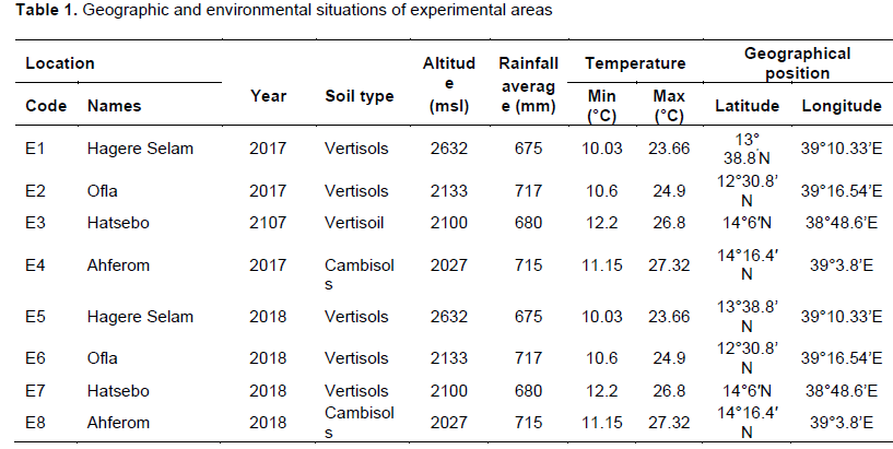
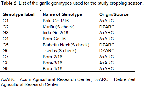
The field experiments were conducted in four diverse garlic growing environments in Tigray region, northern Ethiopia (Ahferom, Hagere selam, Hatsebo and Ofla). The study areas represent low to high altitudes and vary in agro-ecological conditions (Table 1). The genotypes were obtained from Debre Zeit Agricultural Research Center and Axum Agricultural Research Center (Table 2). The experimental design used was a randomized complete block with three replications at each location and year. The experimental plots consisted of 6 rows of 3 m length each. Row-to-row and plant-to-plant distances were kept at 30 and 10 cm, respectively at all the locations. The genotypes were planted in the first week of November for two consecutive years (2017 to 2018/2019) under irrigation. Di-ammonium phosphate (DAP) as a source of phosphorus was applied at the rate of 200 kg ha-1 during planting and nitrogen fertilizer was applied in the form of Urea at the rate of 150 kg ha-1 in splits, half during transplanting and the rest as side dressing at 45 days after transplanting. Furrow irrigation method, scheduled at 8-12 days interval (AxARC, 2016) was used. Weeding and other management practice have been accomplished as required for each site. Data were recorded on 90% physiological maturity, plant height, bulb diameter, bulb weight, number of cloves per bulb and bulb yield per hectare. The yield harvested from four central row of each net harvestable plot in kg was once transformed into tha‑1.
Statistical analysis
The analysis of variance was carried out for each location over two years using SAS version 9.2 (SAS, 2008) and before combining the data, the assumption of (ANOVA) normality test was executed the for bulb yield. Mean comparison was executed using LSD at 5 and 1% level of significance. Genotype -by- environment interaction impact that was detected in ANOVA table that led to the GEI and stability analysis to be done using AMMI and GGE biplot (Yan, 2001). AMMI analysis was performed following the AMMI model in accordance to Gauch (2013) using R software model 3.4.4. The AMMI stability values (ASV) were calculated as advised via Dagnachew et al. (2014). GGE biplot analysis, on the other hand, was used to carry out the usage of the genotype via environment analysis in R software v3.4.4 (Yan et al., 2000; R Team, 2018; Habte et al., 2019). Thus, the first two principal components (PC1 and PC2) were used to graphically represent the GEI, to become aware of the rank of studied genotypes and environments (Yan et al., 2000). The AMMI statistical model is given below:
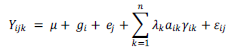
Where: Yijk the yield of the ith genotype in the jth environment, μ the grand mean, gi the mean of ith genotype minus the grand mean, ej the mean of jth environment minus the grand mean, λk is the square root of the eigen value of the principal component analysis (PCA) axis, aik and γjk are the principal component scores for PCA axis n of the ith genotype and jth environment and εij is the error. According to Zobel et al. (1988), AMMI with only two interaction principal component axes could be the best predictive model. Hence, two IPCAs were adopted in this study in AMMI analysis. AMMI stability value (ASV) was calculated to quantify and rank of genotypes. This was carried out using the formula below which is suggested by Purchase (1997). The AMMI stability value (ASV) described by Purchase et al. (2000):
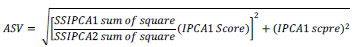
Where:  represents the weighted value assigned to the first interaction principal component score due to its high contributions in the GE model,SSIPCA1 and SSIPCA2 are the sum squares of for IPCA1 and IPCA2 ,respectively. And also IPCA1 and IPCA2 are the first and second IPCA scores for each genotype. The larger ASV the more specifically adapted the genotype is to a certain environment and the smaller ASV indicates a more stable genotype across environments (Purchase, 1997; Ngailo et al., 2019). The GGE biplot were constructed from the first two principal components (PC1 and PC2) derived by subjecting the environment centered yield data (which contains G and GE) to singular valued composition (SVD) (Yan, 2000; Yan et al., 2007). Based on singular value decomposition of the first two principal components, is:
Yij – µ – aj = e1 b1 cj1 + e2 b2 cj2 + εij
Where, Yij is the measured mean of genotype i in environment j, µ is the grand mean, aj is the main effect of environment j, i +aj is the mean yield across all genotypes in environment j, e1 and e2 are the singular values for the first and second principal components, respectively b1 and b2 are eigenvectors of genotype i for the first and second principal components, respectively, cj1 and cj2 are eigenvectors of environment j for the first and second principal components, respectively, εij is the residual associated with genotype i in environment j. AMMI and GGE biplot were performed using R software program Version 3.4.4.
Yield stability index (YSI) and Rank-Sum (RS)
The new approaches known as YSI and RS were calculated by the following formulas:
YSI = RASV + RY
Where RASV is the rank of AMMI stability value and RY is the rank of mean bulb yield of genotypes (RY) across environments. YSI incorporate both mean yield and stability in a single criterion. Low value of this parameter shows desirable genotypes with high mean
yield and stability. Rank sum (RS) = Rank mean (R) + Standard deviation of rank (SDR). RS incorporate both yield and yield stability in a single non-parametric index. Genotypes with the least RS are considered stable with high bulb yield under irrigated conditions. Standard deviation of rank (SDR) was measured as:
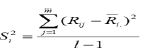
Where Rij is the rank of Xij within the jth environment, Ri. (R), is the mean rank across all environments for the ith genotype and SDR= (S2i) 0.5.
RESULTS AND DISCUSSION
Analysis of variance
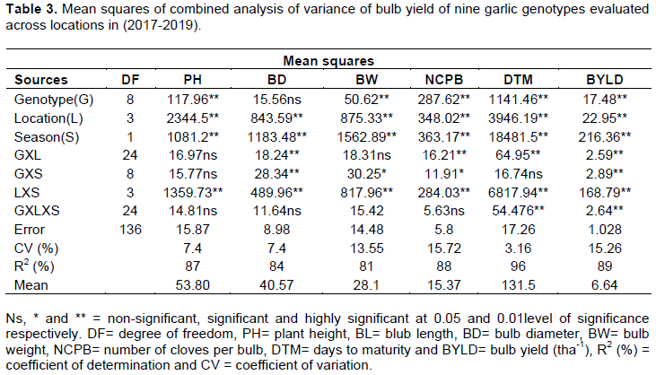
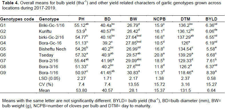
The combined analysis of variance (Table 3) for bulb yield and yield related traits showed highly significance differences (P≤0.01) among genotypes, locations and presence of significance G×E interaction, indicating variation of environments and the presence of genetic variability among genotypes. The analysis of variance also indicated that there was highly significant variation (P<0.01) among the genotypes in plant height (cm), bulb diameter (mm), bulb weight (g), number of cloves per bulb, days to 90% physiological maturity and bulb yield (tha‑1). This showed variability among the genotypes for these characters. The overall mean bulb yield of the locations was ranged from 5.58 to 8.39 tha‑1 (Table 4), therefore, the eight environments (Location × year) showed broad variation in their yield production potential. The mean bulb yield of genotypes was 6.64 tha‑1 (Tables 3 and 4). The performance of genotypes in all yield associated characteristics was different both in each and throughout locations. This indicated that the efficiency of a breeding program aimed only at yield enhancement resulted in inconsistent performance of genotypes due to significant genotype- by- environment interaction effect, which complicates the procedure of crop variety development particularly when varieties are chosen in one environment and used in others (Singh et al., 2016).
AMMI analysis of variance for bulb yield
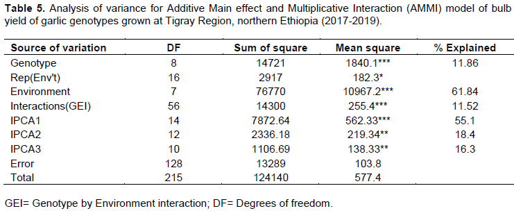
Combined analysis of variance for bulb yield of the nine garlic genotypes examined across eight environments is presented in Table 5. The main effect differences among genotypes, environments, and the interaction results were highly significant (P < 0.01) of the whole variance of bulb yield. The environment impact accounted for 61.84%, whereas genotype and G × E interaction results accounted for 11.86 and 11.52% of the total variation, respectively (Table 5). The maximum environmental sum square indicated that there was a huge difference among the testing locations causing unique genotypes to perform in another way across the testing environments and the excessive percentage of the environment is an indication that the main factor that influence yield performance of garlic genotypes in Ethiopia is the environment. Genotypes revealed highly significant (P<0.001) variations for bulb yield. This shows that there was genetic difference among genotypes for this trait. This variation is beneficial when intending to find out about the consequences of G×E interaction, as properly as to consider the phenotypic stability of genotypes. The magnitude of the GEI sum of squares used to be rather similar with that of the genotypes, indicating that there was by some means comparable response of some of the genotype across environments.
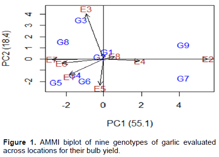
The results of AMMI model for bulb yield are presented in Table 5. As it is viewed from Table 5, the mean square of the three IPCA was highly significant (P<0.001). The AMMI biplot, which accounted for 73.5% of the G×E interaction, gives the interaction principal component rankings of the 1st and 2nd IPCA. The first PC axis (PC1) score explained 55.1% of the variant in GEI, while the 2nd PC axes accounted for18.4% of the variability. Many researchers witnessed that the best accurate AMMI model prediction can be made by using the first two IPCAs (Yan et al., 2000). Therefore, the dataset obtained from the interaction of 9 genotypes examined at eight environments were well predicted through the first two IPCAs. On the other hand, the IPCA scores of a genotype in the AMMI analysis are indication of the stability of a genotype throughout environments (Purchase, 1997). Accordingly, the closer the IPCA scores to zero (origin), the more stabile the genotypes are across all environments (Purchase, 1997). The IPCA1 used to be plotted on x-axis whereas IPCA2 was plotted on y-axis for bulb yield and yield components (Figure 1). The greater the IPCA scores (positive or negative) as it is a relative value, the greater especially adapted a genotype is to certain environments. The greater IPCA scores approximate to zero, the more stability the genotype is throughout environments sampled (Purchase, 1997). The IPCA1 and IPCA2 rankings of bulb yield for each genotype and the corresponding AMMI stability value (ASV) are presented in Table 6. According to ASV ranking, genotype 2 had the lowest value indicating its high stability, while genotypes 9 and 7 were extraordinarily unstable. Purchase (1997) pointed out that the closer the genotypes score to the center of the biplot the genotype is broadly adapted and the reverse is true. Regarding the position of the environments in the biplot graph, locations E2 (Ofla) and E4 (Ahferom) were the most discriminating environments as they have long distance between their marker and the biplot origin (Figure 1). However, due to their massive IPCA2 score, genotypic variations discovered at these environments may not precisely show the genotypes average yield across locations. The interaction principal component one (IPCA1) and the interaction principal component two (IPCA2) scores in the AMMI model are indications of stability.
Considering the first interaction principal component (IPCA1), the genotype G5, was the most stable genotype with IPCA1 value (-2.53). When the second interaction principal component (IPCA2) was considered, G5 was the most stable genotype with interaction principal component value (-2.07) followed by the genotype G6 with the IPCA2 value (-1.94). The two principal components have their own extremis, however calculating the AMMI ASV is a balanced measure of stability (Purchase, 1997). The genotype with lower ASV values is viewed stable and genotypes with higher ASV are unstable. Based on the value of ASV, genotype G2 was the most stable with an ASV value of 0.67 followed with the genotypes G1 and G6 with ASV value of 0.84 and 3.59 of bulb yield respectively. Genotypes G7, G9 and G5 were the most unstable with ASV value of 12.71, 12.64 and 7.86 of bulb yield respectively (Table 6).
Yield stability index (YSI)
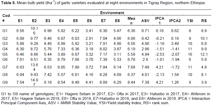
Stability is not the only criterion for selection, due to the fact that most stable genotypes would no longer necessarily provide the best yield across environments (Mohammadi et al., 2010), consequently there is a need for approaches that comprise both mean yield and stability in a single index number of authors introduced extraordinary standards for simultaneous selection of yield and stability rank-sum, modified rank-sum and yield stability (Farshadfar et al., 2011). In this regard, ASV takes into account both IPCA1 and IPCA2 and justifies most of the variation in the GEI. The genotype with least YSI is regarded as the most stable with high yield mean. It was utilized to identify high yielding and stable genotypes in cereal crops like durum wheat (Mohammadi et al., 2010). Based on YSI, the most stable genotype with high bulb yield is genotype G9 with YSI of 9 accompanied via G7 and G6 YSI of 11 and 11, respectively .The highest YSI indicate that G4, G5 and G8 were unstable genotypes. Rank-sum (RS) showed that genotype G9 produced high bulb yield and followed via genotype G7 indicating that they were the most stable genotypes with high bulb yield. Both YSI and RS confirmed that genotype G7 gave high bulb yield.
Analysis of GGE biplot for bulb yield
GGE Biplot analysis shows “which-won-where” pattern, ranking of cultivars on the basis of yield and stability, and correlation vectors among environments. Angles between environment vectors were used to judge correlations (similarities/dissimilarities) between pairs of environments (Yan and Kang, 2003; Yan, 2011). GGE biplot is visualized on the basis of consequences defined for the first two principal components (Yan et al., 2001). In the current study, the first two principal components of GGE biplot explained 84.13% (PC1=74.52 and PC2=9.61%) of the whole variations (Figure 2). In the polygon, genotypes located far away from the origin are the vertex genotypes having the highest yield in the region (Esayas et al., 2019; Habte et al., 2019). In this study, genotypes G9, G7, G5 and G3 had the highest yield in their respective sector.
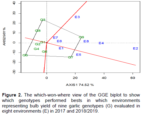
The GGE Biplot graphic analyses of the nine garlic genotypes tested at eight environments are presented in Figure 2. Rays in Figure 2 divided the biplot into four sectors. The environments were located in two mega-environments where group 1 contained environments E2,E3,E4, E6, E7 and E8 and group 2 had two environments E1 and E5 (Figure 2), while the genotypes were located in all four sectors. The genotypes found at vertex of the sectors are the most profitable genotypes of that sector (Yan and Tinker, 2006).The genotype on the vertex of the polygon, contained in a mega-environment, had the highest yield in at least one environment and was one of the best-performing genotypes in the other environments (Yan, 2002). Accordingly, the vertex genotype G9 (Bora-1/16) was high yielder in most of environments except E1 and E5 where G7 (Bora-2/16) was the winner. Therefore, genotype G9 was best yielder in environments E2, E3, E4, E6, E7 and E8. Genotype 7 gave highest yield in E1 and E5 (Figure 2 and Table 6). The other vertex genotypes (G3 and G5) were not the highest yielding genotypes at any environment. Thus genotypes G9, G7, G3 and G5 are specifically adapted. G1 and G2 genotypes were closest to the center of origin; therefore they were broadly adapted genotypes.
Relationship among environments and discriminative vs. representativeness
The vector view of a GGE biplot provides a summary of the interrelationships among the environments (Yan, 2002). Provided that the biplot explained an adequate amount (≥50%) of the total variation, the correlation coefficient between any two environments is reliable (Yan et al., 2000). Furthermore, the length of an environmental vector is an estimation of discriminating power of the environment (Yan et al., 2007). Accordingly, the results of the present study revealed that the first principal component (PC1) and the second (PC2) respectively clarified 74.52% and 9.61% of the variance (Figure 3). The two principal component axis (PC1 and PC2) together clarified 84.13% of the total variance. So this biplot can be used for extracting interrelationships among the environments.
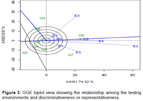
A long environmental vector represents a high capacity to discriminate the genotypes. With the longest vectors from the origin, environment E2 was the most discriminating of the genotypes, while E3, E4, E5 and E8 were moderately discriminating. However, with the shortest vector from the origin, E7 provided little or no information about the genotype differences. Furthermore, the vector view of the GGE-biplot provides a brief summary of the interrelationships among the environments. Two environments are positively correlated if the angle between their vectors is <90°, negatively correlated if the angle is >90°, independent if the angle is 90° (Yan and Tinker, 2006). Based on this, E2, E4, E6, E7 and E8 environments were positively correlated because all of the angles among their vectors were smaller than 90°. However, the angle between vectors of tester E3 andE1, E3 and E5 were approximately 90°, and were not correlated (Figure 3).
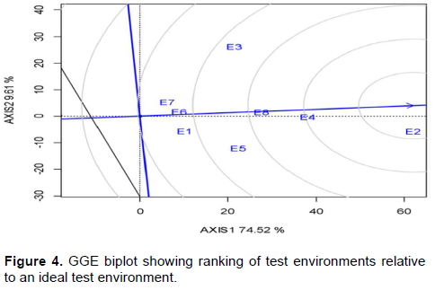
Ranking testing environments relative to the ideal environment and genotype
Average environmental axis (AEA) is a line passing via the origin and pointing to the positive direction with its distance equal to the longest vector. An ideal environment is representative and has the highest discriminating power (Yan and Tinker, 2006). The ideal environment is located in the first concentric circle in the environment-focused the GGE biplot and the environments that are close to the ideal environment are defined as the desired environments. Based on this, E2 located in the first concentric circle and has been the most ideal environment (Figure 4). Thus, genotype evaluation in E6 environment maximized the observed genotypic variation among genotypes for bulb yield of the tested garlic genotypes. E4 and E8 environments were close to the ideal environment (E2) and these environments were identified as suitable environments. This difference between environments can be related to soil fertility, climate changes and other environmental variations from year to year. The most acceptable is the one closest in the sketch of the ideal environment (Yan et al., 2000). The environments E2 (Ofla, 2017), E4 (Ahferom, 2017) and E8 (Ahferom, 2018) contained in the third concentric circle is the place with best potential to discriminant genotypes, favoring the choice of ideal genotypes (Figure 4 and Table 6).
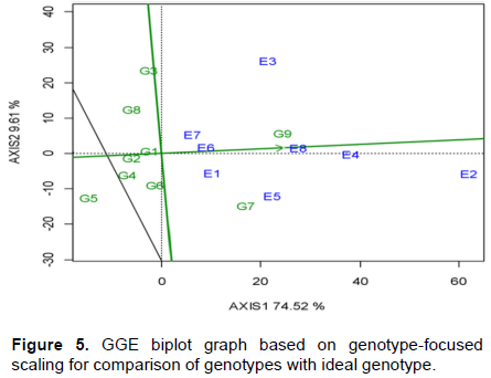
Ranking genotypes relative to the ideal genotype and environment
An ideal genotype is defined as the one with the highest yield across the test environments and is definitely stable in performance (Yan and Kang, 2003). The average environment coordination view of the GGE biplot suggests the rating of genotypes primarily based on the overall performance of best genotypes (Figure 5). The relative adaptation of the best genotype is evaluated through drawing a line passing via the biplot origin and the best genotype marker. This line is referred to as a genotype axis and is related to the economic profitable genotype (Habte et al., 2019). Such ranking of genotypes revealed that both G9 and G7 are the high yielding genotypes.
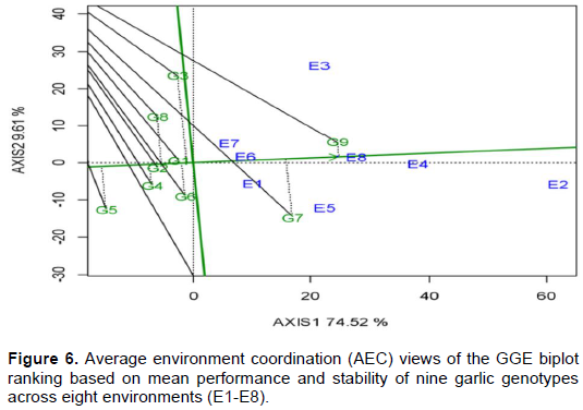
Genotypes mean yield vs. stability
The mean yield performance and stability of genotypes was evaluated by an average environment coordination (AEC) method (Yan, 2001, 2002). In the AEC system, AEC X axis (PC1) passes through the biplot origin with an arrow indicating the positive end of the axis and indicates the mean performance of genotypes. The ATC Y-axis passes through the biplot origin and is perpendicular to the ATC X-axis. This axis indicates the stability axis (PC2) (Figure 6). Based on these, statistically, the stable genotypes located near the AEC X axis (PC1) with PC2 scores of almost zero. According to Figure 6, genotypes with above average yield were G9 and G7 and located on the right side of the biplot origin, while genotypes with blow average yield were G3, G5 and G8 and located on left side of the biplot origin. A best genotype for a particular environment has the best possible mean yield and responds best at that unique environment while it is less stable in the other environments and wants to be proposed for a specific environment (Yan et al., 2001). According to the similar authors, best cultivars have large PC1 rankings (high mean yield) and small PC2 scores (high stability). Thus, in the present study, G9 and G7 which had higher PC1 and smaller PC2 rankings had been recognized as high yielding and stable. Therefore, the genotypes G7 and G9 with stable and high yield can be recommended as commercial variety for the Tigray region and others which have similar agro-ecology.
CONCLUSION
From the current study, it is concluded that multiple methods were employed to analyze stability. The AMMI and GGE biplot methods can be effectively utilized for the identification of the suitable genotypes for suitable environments. The results of AMMI analyses indicated that garlic bulb yield performances was highly affected by environmental effect followed by the magnitude of GEI, but genotype contributed the minimum effect. The AMMI and GGE biplot analysis permitted estimation of interaction effect of a genotype in each environment and they helped to identify genotypes best suited for specific environments. The GGE biplot analysis shown that the genotypes G9, G7, G5 and G3 were corner genotypes and suited to specific environments. The polygon views of the GGE biplot grouped in two possible mega environments. The first mega environment consisted of six environments (E2, E3, E4, E6, E7 and E8); and the second mega environment consisted of two environments (E1 and E5). In addition, the discriminating power vs. representativeness view of the GGE biplot has been an effective tool for test environments evaluation. Environment E2 (Ofla) and E4 (Ahferom) were the most discriminating for bulb yield of the tested garlic genotypes. According to the AMMI and GGE biplot models, considering simultaneous average yield and stability, G9 (Bora-1/16) and G7 were the best genotypes. Therefore, these genotypes should be released for Tigray region and others similar agro-ecologies to enhance the productivity of garlic.
CONFLICT OF INTERESTS
The authors have not declared any conflict of interests.
ACKNOWLEDGMENTS
The authors grateful appreciate the Tigray Agricultural Research Institute (TARI) and Axum Agricultural Research Center (AxARC) for financial support and are also indebted to Horticulture staffs at Alamata Agricultural Research Center and Mekelle Agricultural Research Centers for provision of experimental fields, technical support and data collection during the experiments were conducted.
REFERENCES
|
Batth GS, Kumar H, Gupta V, Brar PS (2013). GGE Biplot Analysis for Characterization of Garlic (Allium sativum L.) Germplasm Based on Agro-Morphological Traits. International Journal of Plant Breeding 7(2):106-110. |
|
|
Brewster JL (1994). Onions and other Vegetable Alliums. CABI publishing Wellesbourne, UK. |
|
|
CSA (Central Statistical Agency). (2017). Agricultural sample survey Report on area and production of major crops of private peasant holdings. The FDRE Statistical bulletin 1:584. Addis Ababa, Ethiopia 118p. |
|
|
Dagnachew L, Masresha F, Santie de V, Kassahun T (2014). Additive Main Effects and Multiplicative Interactions (AMMI) and genotype by environment interaction (GGE) biplot analyses aid selection of high yielding and adapted finger millet varieties. Journal of Applied Biosciences 76(1):6291-6303. |
|
|
Dejen B (2018). Review on the Application of Biotechnology in Garlic (Allium Sativum) Improvement. International Journal of Research Studies in Agricultural Sciences 4(11):23-33. |
|
|
Diriba-Shiferaw G (2016). Review of management strategies of constraints in garlic (Allium sativum L.) production. Journal of Agricultural Sciences -Sri Lanka 11(3). |
|
|
Esayas T, Frehiwot G, Hussein M, Melaku T, Diribu T, Abebech S, (2019). Genotype× environment interaction by AMMI and GGE biplot analysis for sugar yield in three crop cycles of sugarcane (Saccharum officinirum L.) clones in Ethiopia. Cogent Food and Agriculture 5:1-14. |
|
|
Farshadfar E, Mahmodi N, Yaghotipoor A (2011). AMMI stability value and simultaneous estimation of yield and yield stability in bread wheat (Triticum aestivum L.). Australian Journal of Crop Science. 5(13):1837-1844. |
|
|
Gauch HG, Piepho, HP, Annicchiaricoc P (2008). Statistical analysis of yield trials by AMMI and GGE. Further considerations. Crop Science 48:866-889. |
|
|
Gauch HG (2013). A simple protocol for AMMI analysis of yield trials. Crop Science 53:1860-1869. |
|
|
Gauch HG (2006). Statistical analysis of yield trials by AMMI and GGE. Crop Science 46:1488-1500. |
|
|
Gauch HG, Zobel RW (1997). Identifying MegaEnvironments and Targeting Genotypes. Crop Science 37:311. |
|
|
Getachew T, Asfaw Z (2010). Achievements in shallot and garlic research. Report No.36. Ethiopian Agricultural Research Organization, Addis Ababa Ethiopia. |
|
|
Habte J, Kebebew A, Kassahun T, Kifle D, Zerihun T (2019). Genotype-by-Environment Interaction and Stability Analysis in Grain Yield of Improved Tef (Eragrostis tef) Varieties Evaluated in Ethiopia. Journal of Experimental Agriculture International 35(5):1-13. |
|
|
Mohammadi R, Mozaffar RM, Yousef A, Mostafa A, Amri A (2010). Relationships of phenotypic stability measures for genotypes of three cereal crops. Canadian Journal of Plant Science 90:819-830 |
|
|
Mohammed A, Shiberu T, Thangavel S (2014). White rot (Scelerotium cipivorum Berk)-an aggressive pest of onion and garlic in Ethiopia: an overview. Journal of Agricultural Biotechnology and Sustainable Development 6(1):6-5. |
|
|
Ngailo S, Shimelis H, Sibiya J, Mtunda K, Mashilo J (2019). Genotype-by-environment interaction of newly-developed sweet potato genotypes for storage root yield, yield-related traits and resistance to sweet potato virus disease. Heliyon, Elsevier 5(3):1-23. |
|
|
Purchase JL, Hatting H, Van Deventer CS (2000). Genotype × environment interaction of winter wheat (T. aestivum) in South Africa: Stability analysis of yield performance. South African Journal of Plant Soil 17(3):101-107. |
|
|
Purchase JL (1997). Parametric analysis to describe genotype x environment interaction and yield stability in winter wheat, University of Free State. Bloemfontein, South Africa |
|
|
R Team (2018) R: a language and environment for statistical computing. R Foundation for Statistical Computing, Vienna. |
|
|
SAS Institute Inc. (2008). SAS/STAT ®9.2 User's Guide. Cary, NC: SAS Institute Inc |
|
|
Singh RK, Dubey BK, Gupta RP (2016). Genotype × environment interaction and stability analysis for yield and its attributes in garlic (Allium sativum L.). Journal of Spices and Aromatic Crops 25(2):175-181. |
|
|
Tewodros B, Fikreyohannes G, Nigussie D, Mulatua H (2014). Registration of 'Chelenko I'Garlic (Allium sativum L.) Variety Haramaya University, Ethiopia. East African Journal of Sciences 8(1):71-74. |
|
|
Yan W (2001). GGE biplot: A windows application for graphical analysis of multi environment trial data and other types of two-way data. Agronomy Journal 93:1111-1118. |
|
|
Yan W (2002). Singular value partitioning in biplot analysis of multi-environment trial data. Agronomy Journal 94:990-996. |
|
|
Yan W (2011). GGE Biplot vs. AMMI Graphs for Genotype-by-Environment Data Analysis. Journal of the Indian Society of Agricultural Statistics 65(2):181-193. |
|
|
Yan W, Tinker NA (2006). Biplot analysis of multi environment trial data: Principles and applications. Canadian Journal of Plant Science 86:623-645 |
|
|
Yan W, Kang MS (2003). GGE Biplot analysis: a graphical tool for breeders, geneticists, and agronomists. Boca Raton, FL: CRC Press. |
|
|
Yan W, Cornelius PL, Crossa J, Hunt LA (2001). GGE Biplot analysis of multi-environment trial data. Crop Science 41(3):656-663. |
|
|
Yan W, Hunt LA, Sheng Q, Szlavnics Z (2000). Cultivar evaluation and mega environment investigation based on the GGE biplot. Crop Science 40:597-605. |
|
|
Yan W, Kang MS, Ma B, Wood S, Cornelius PL (2007). GGE biplot vs. AMMI analysis of genotype-by environment data. Crop Science 47:643-655. |
|
|
Yan W, Wu HX (2008). Application of GGE biplot analysis to evaluate genotype (G), environment (E), and G× E interaction on Pinus radiata: A case study. New Zealand Journal of Forestry Science 38(1):132-142. |
|
|
Zobel RW, Wright MJ, Gauch HG (1988). Statistical analysis of a yield trial. Agronomy Journal 80:38. |
|
Copyright © 2024 Author(s) retain the copyright of this article.
This article is published under the terms of the Creative Commons Attribution License 4.0


