ABSTRACT
Access to quality drinking water is of major concern for sustainable development in developing countries with regard to physico-chemical properties. Groundwater from shallow wells is the main source of domestic water supply for the community of Ainabkoi Sub-County of Uasin Gishu County in Kenya. Seasonal agricultural production activities expose the water to possible pollution. In this regard the study aimed to assess the seasonal physico-chemical parameters in shallow wells among different farm sizes in three wards within Ainabkoi sub-county. Each ward was a homogenous stratum of same size-ranged farms classified as large, medium and small farm sizes in Ainabkoi, Olare and Kaptagat (Kipsinende) wards respectively. Within each ward farms were purposively and randomly selected such that only accessible farms that had access to either a privately owned or communal wells were selected. Wells were sampled during the wet and dry seasons of the year for a period of two years. The seasonal levels of physico-chemical parameters pH, Electrical Conductivity (EC), Total Dissolved Solids (TDS), Dissolved Oxygen (DO), Total Suspended Solids (TSS), turbidity and temperature were determined. There were non-significant differences between the farm sizes in the groundwater pH, EC, DO, turbidity and temperature. The groundwater pH values were within the WHO standards range of 6.3 to 8.5. EC values were below the recommended limits of potable water of 250 µccm-1. TDS and TSS differed significantly between farm sizes. Wells within the small mixed farm sizes had significantly high TDS levels ranging from 30-250 mgL-1. The TDS values ranged from 32.20-203.30 mgL-1 hence the wells can be classified as fresh water wells. TSS values were significantly higher during the wet season by about 90% and highest in wells within the large sized farms. The turbidity levels were higher than the recommended limits by WHO of at least 5.0 NTU in areas with limited resource availability. In conclusion, the groundwater in Ainabkoi sub-county can conservatively be categorised as safe for domestic use with regard to physico-chemical parameters.
Key words: Farm sizes, groundwater, season; physico-chemical properties.
Potable or drinking water is defined as having acceptable quality in terms of its physical, chemical, and bacteriological parameters so that it can be safely used for drinking and cooking (Gadgil, 1998). Drinking water quality is of major concern in developing countries with regard to microbiological, inorganic contaminants and physico-chemical properties which deteriorate water quality (Sorlini et al., 2003). Communities should have access to safe drinking water as a basic need to health and sustainable development as outlined in the sustainable development goals (SDGs) which focus on ensuring universal and equitable accessibility of safe water for all by 2030 (6th SDG) (Osborn et al., 2015). However, the chemical and biological quality of water is often overlooked in comparison with the quantity view point of water for drinking, domestic and agriculture use (Falowo et al., 2017). Groundwater is mainly contaminated and polluted by anthropogenic activities such as modern farming and other domestic and industrial activities. Since groundwater is a major source of water for domestic water supply, its quality should therefore be of major concern especially in agricultural settings. World Health Organisation (WHO, 2011) recommends regular physical assessment of water quality especially after heavy rains to monitor any temporal changes in important physical characteristics such as colour, odour, turbidity, taste, temperature, solids and chemical characteristics such as acidity, alkalinity and hardness.
The study was carried within Ainabkoi Sub-County of Uasin Gishu County in Kenya. Groundwater is the main source of domestic water supply for the community and is exploited through shallow wells (Uasin Gishu Integrated Development Plan (UGCIDP), 2013). Groundwater is considered to be more stable in quality hence requiring no treatment unlike surface waters, is conveniently available and accessible for the family and wells can be developed at comparatively low costs. However, the groundwater resource in Ainabkoi is exposed to possible pollution from agricultural production activities which may make it unfit for consumption. Mixed farming agriculture (food/commercial crops and livestock-dairy) characterised by different farm sizes is the predominant economic activity for the rural community of Ainabkoi Sub-County with farmers gradually shifting to intensive horticultural farming (UGCIDP, 2013). For purposes of this study different farm sizes were determined as a working farm typology because it captured common characteristics within farms in each ward within Ainabkoi Sub-County. According to Ojiem et al. (2006) the heterogeneity of farming size is created by several biophysical and socio-economic factors. However, official farm typologies in Africa are almost nonexistence due to general state withdrawal in agricultural public policies (Matus et al., 2013). The selection of factors that define farm typology varies greatly from study to study and may be governed by the purpose of research (Goswami et al., 2014). Therefore farms in Ainabkoi, Kaptagat and Olare wards were classified as large, medium and small farm sizes respectively. There are also concerns with the notable upsurge of chronic diseases such as cancer reported
within the county in the recent past with a total of 5,137 various cancer cases documented between 2004 and 2012 (Kirumba, 2014).
In view of the foregoing and in line with the county objectives and concomitant strategies aimed at improving access to clean and potable water to the community it became imperative to access the seasonal quality of ground water. This will provide base data and information which is largely non-existent, on the water quality status to policy makers for future management and planning. The study therefore examined the seasonal levels of physico-chemical parameters of the well water among different farm sizes in Ainabkoi Sub-County, Uasin Gishu County, Kenya.
Description of the study area
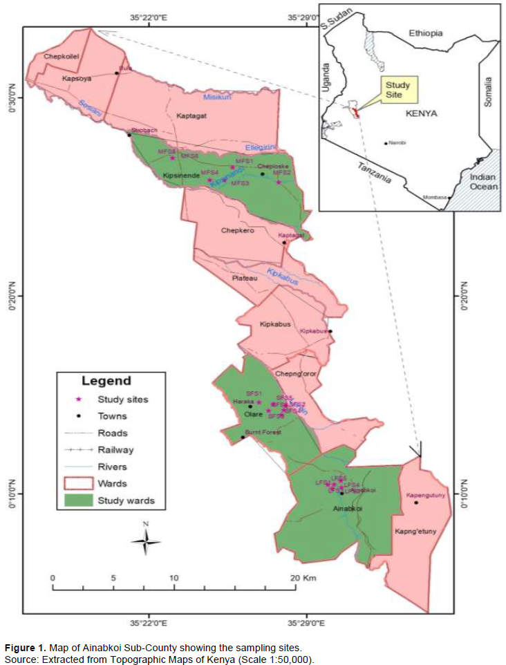
Uasin Gishu County lies between longitudes 34° 50´ East and 35° 37´ West, and latitudes 0° 03´South and 0° 55´ North and with a total area coverage of 3,345.2 km2 and about 202,000 households (UGCIDP, 2013). Uasin Gishu is a highland plateau with a terrain that varies greatly with altitude, ranging between 1500 m above sea level at Kipkaren in the West to 2100 m at Timboroa in the East. There are six sub-counties namely Turbo, Soy, Ainabkoi, Moiben, Kessess and Kapseret in Uasin Gishu (Figure 1). Uasin Gishu is endowed with good land resources and varied agro-ecological potential and is commonly referred to as the bread basket of the country due to the predominant production of rain-fed maize production.
The county has a long cropping season between March and October and intermediate rains which can be divided into two variable cropping seasons. The first rains normally start at the end of March and the second at the end of June. Average rainfall amounts are sufficiently high and range between 624.9 to 1,560.4 mm with two distinct peaks occurring between March-May and June-September and a dry spell occurring between November and February. The study was conducted in 2012 and 2013 in three wards within Ainabkoi sub-county namely Ainabkoi, Olare and Kaptagat (Kipsinende) which have extensive agricultural activities. A baseline reconnaissance farm survey found that farmers predominantly practiced mixed farming whereby they grew maize, kept some farm animals, and had a variety of vegetables and fruit crops in small gardens beside their homes.

However, each farm had its own unique characteristics with regard to the farm sizes, number and types of domestic animals kept, the maize acreage, variety of vegetable and fruit crops grown, and the homestead/ property development such as landscaping, housing, toilet construction, well ownership and construction. In order to conceptualize and establish effective comparison between farms it was necessary to conceive a working typology that captured a common characteristic within farms. It was identified that farms in Ainabkoi ward were mainly large, family-generations-owned mixed farming size and ranged more than 40 acres in size (>40 acres) with privately owned wells. In Kaptagat ward, farms were medium sized (10-40 acres) mixed farms with privately owned wells. The farms in Olare ward were small mixed farm sizes which ranged 2-10 acres in size and with communally owned wells. In view of the foregoing, the three wards were identified as non-overlapping strata and farms were stratified on the basis of farm sizes into three farm typologies. Each ward was therefore considered as a stratum of homogenous farms characterised by individual farm sizes with the same extensiveness or size in terms of acreage and accessibility to a well. Purposive random sampling technique was applied in selection of the representative farms within each ward whereby only accessible farms that had access to a well for evaluation of the groundwater sources were selected. Five farms in each ward were therefore identified for well water sampling. Hence a total of 15 wells were sampled during the wet and dry seasons of the year for a period of two years. The well coordinates in Ainabkoi ward were within the latitude range of 0°10’19.4”N to 0°10’33.9”N and longitudes 35°30’03.9”E to 35°30’34.9” E. In Kipsinende ward the well coordinates ranged from 0° 25’ 45’’N to 0° 26’ 59’’N and 35° 23’ 4’’E to 35° 27’ 47’’E and in Olare from 0° 14’ 8’’N to 0° 14’ 38’’N and 35° 26’ 55’’E to 35° 28’ 6’’E. The rain or wet season (WS) usually occurs as from March to August while the dry season (DS) is from November to February. It was assumed that the possible variations due to the unpredictable cause-effect impact chain of the agroecosystems and the environment were negligible and that the interaction between farm sizes and year had no agronomic meaning and was therefore less important than the interaction between farm sizes and season. Therefore repetition over seasons was preferred to repetition over years.
Water sample collection
Groundwater samples were collected at least every week from just before planting, in January to March, during planting in April and through to two weeks after topdressing in June-July and thereafter at least once a month until after harvesting in October in 2012 and 2013. Sampling of groundwater was also done at least once a month during off production season in the months of November to January. The purpose of the sampling times were aimed at monitoring any possible temporal changes in groundwater characteristics throughout the production cycle and during off season. Groundwater sampling was done in triplicates at each sampling time, directly into clean high density 150 ml polyethylene
bottles, sealed and stored in an icebox in the field and transported to the laboratory within the same day. Samples were transported immediately to Kenya Marine Fisheries research institute, (KMFRI) laboratories and kept frozen prior to analysis.
It was expected that the nutrient levels in the water samples would not be significantly changed through freezing since it is considered an effective means of nutrient preservation in water samples (Fellman et al., 2008). Unstable hydrochemical parameters such as pH, Electrical Conductivity (EC) and Total Dissolved Solids (TDS) were measured in situ (in the field) immediately after collection of samples while the others were analysed in the laboratory as described by the American Public Health Association (APHA, 1995).
Determination of pH, EC and TDS
The pH, EC and TDS parameters were measured in-situ using a combined pH/EC/TDS combo (Hanna instruments) Model HI 98130 by selecting the target mode. The probe was submerged into the sampled water and readings taken when they stabilised. Any electromagnetic interference was minimised by using plastic bottles to hold the water samples. TDS was then determined by the method of O'wen (1979), by multiplying the EC value of the water sample by 0.65.
Dissolved oxygen
Dissoloved oxygen was determined by using the Winkler’s method according to APHA (1995).
Total suspended solids (TSS)
The concentration of total suspended solids was estimated gravimetrically on glass-fibre filters (Whatman GFC, or Ederol BM/C filters) after drying to constant weight at 95°C (APHA, 1995).
Turbidity
Turbidity was measured using a Hatch Turbidimeter 2100 P (APHA, 1995). Turbidity is the cloudiness of water as a result of suspended material such as clay, silt, organic/soluble organic, planktonic, microscopic organism thereby inhibiting light transmission by scattering and absorption rather than being transmitted in a straight line (APHA, 1995).
The comparison of the mean values for the physico-chemical characteristics of groundwater in the different farm size in 2012 and 2013 are shown in Table 1. There were non-significant differences between the farm size in the water pH, DO, EC, turbidity and temperature. However, there were highly significant differences between the farm sizes in the TDS and the TSS. The small farm size had significantly the highest TDS compared with the large and medium mixed farm size. The TSS levels were significantly highest in the large farms size and least in the small mixed farm size. Turbidity was the only physico-chemical characteristic in the wells that exceeded the permissible levels by World Health Organisation (WHO, 2011) of at least less than 5 NTU in rural supplies. The average turbidity levels in the sampled well water were 86.67 NTU. The average values of the groundwater physiochemical characteristics were determined and compared for the wet and dry seasons of 2012 and 2013 (Table 2). There were no significant seasonal differences between the wet and dry seasons in the pH, EC, TDS and Turbidity in the groundwater.
pH
The pH of the groundwater samples in all the farm size ranged from 5.94 to 8.96 in 2012 with an average of 7.41 and 6.6 to 8.96 with a mean of 7.49 in 2013. The pH of the groundwater samples ranged from 5.94 to 8.66 during the wet season with a seasonal average pH of 7.43 and from 6.46 to 8.96 with a mean value of 7.87 in the dry season (Table 2). However, it was observed that the pH fluctuated considerably within each individual well throughout the production cycle. The general trend observed was that most wells had a pH level averaging about 7.5 with a few wells within the medium and small mixed farm size that had pH levels of 8.0 during the wet and dry season.
Dissolved oxygen (DO)
The DO levels in the groundwater samples ranged from 3.01 to 8.79 mgL-1. There were no significant differences in the dissolved oxygen levels between the wells in the different farm sizes (Table 1). However, there were significant differences in the DO levels in the wet and dry seasons (Table 2). The DO ranged from 3.90 to 8.72 mgL-1 with a mean of 6.75 mgL-1 during the wet season and from 3.01 to 8.79 mgL-1 in the dry season with a mean of 6.51 mgL-1. These results indicate that the DO levels were higher during the wet season than the dry season by a margin of 3.7%.
Electrical conductivity (EC)
The EC values in the groundwater samples ranged from 5.32 to 290 µc cm-1. The ANOVA showed that there were no significant differences in EC values between the farm size (Table 1) and also no-significant seasonal variations in the EC values (Table 2). The conductivity of the water samples varied from 38.77-146 μScm-1 with a seasonal average of 88.21 μScm-1 during the wet season, while it varied from 5.32-290 μScm-1 during the dry season and a seasonal average of 91.35 μScm-1.
Total suspended solids (TSS)
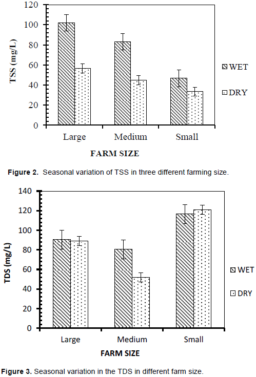
There were highly significant differences in TSS between the wells in the different farm sizes (Table 1). The TSS were highest in wells within the large farm size with values varying from 8.67-247.1 mgL-1. The TSS values in well water on average ranged from 12.2-273.5 mg/L in the medium farm size and 9.2-150.3 in the small farm size. The TSS values were significantly higher during the wet season than during the dry season by about 90% (Table 2). The TSS concentration during the wet season was highest in wells within the large farm size, and lowest in wells in the small farm size (Figure 2).
Total dissolved solids (TDS)
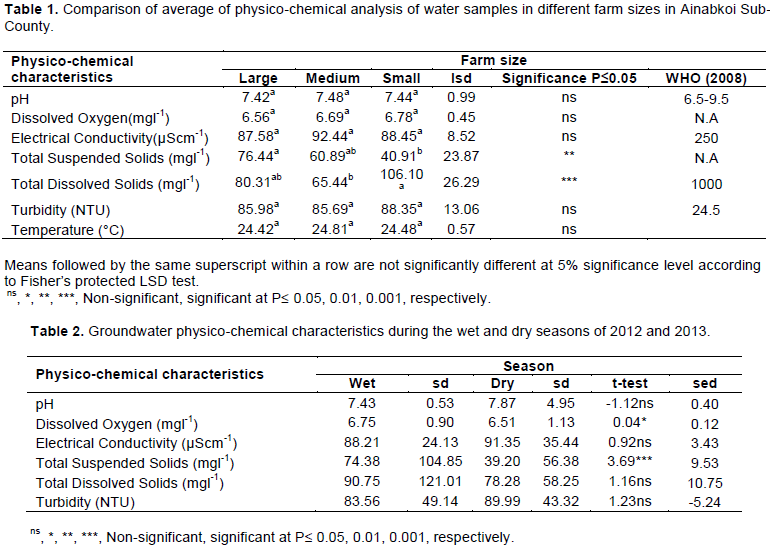
Analysis of variance showed highly significant differences between well water samples in the different farm sizes (Table 1). Wells within the small mixed farm size had significantly the highest levels of TDS ranging from 30-250 mgL-1 and averaging 119 mgL-1 (Figure 3). The content of TDS in well water in the large farm size ranged from 33-168 mgL-1 with an average of about 90 mgL-1, while in the medium farm size TDS concentration ranged from 10-188 mgL-1 with an average of 66 mgL-1. There were non-significant seasonal differences in TDS levels in well water (Table 2). The seasonal TDS values ranged from 32-202 mgL-1 during the wet season and 58-136 mgL-1 during the dry season. The TDS in the well water did not exceed the maximum allowed limit of 1000 mgL-1.
Turbidity
There were no significant differences in turbidity between the farm sizes (Table 1). The turbidity averaged across the farm size varied from the lowest value of 22.5 to the highest record of 119.9 NTU. There were non-significant seasonal differences in the turbidity level of the sampled well water. The average turbidity levels ranged from 22.7-119.9 NTU with a mean of 70 NTU and 20.4-113 NTU with a mean of 76 NTU were during the wet and dry seasons respectively.
The pH values in the sampled groundwater were within the WHO standards of 6.5 to 8.5 (WHO, 2011). The optimum pH required will vary in different supplies according to the composition of the water and the nature of the construction materials used in the distribution system, but it is usually in the range 6.5-8.5. Anim-Gyampo et al. (2014) reported closely similar results whereby borehole water pH ranged between 5.77 and 8.3. These results therefore indicate that the well water samples represented satisfactory water pH values for drinking and domestic water use. Seasonal pH variations showed that the average pH values were slightly lower during the wet season (pH 7.4) than during the dry season (pH 7.5). These results concur with those reported by Olutona et al. (2012) who reported lower pH of 7.25 during the wet season and 8.08 during the dry season, an indication of lower levels of hydrogen ions. According to Hounslow’s classification of wells, (Hounslow, 1995) as being either moderately acidic (4-6.5), neutral (pH 6.55-7.8) or alkaline (pH 7.8-9), 71% of the wells in 2012 and 54% in 2013, can be classifed as being neutral pH (pH 6.5-7.8). According to the classification, on average only 4.5% and 4% of the wells were moderately acidic (pH 4-6.5) during the wet and dry seasons respectively. Although there are no health-based drinking water standards for pH, an optimum pH of 6.5-9.5 is recommended (WHO, 2008). The united States of America Environemental Protection Agency (USEPA) has established a secondary standard for pH range of 6.5-8.5, because pH within this range can produce aesthetic effects such as staining and scaling of eqipment and lead to dissolved concentrations of some metals associated with health effects (Fisher et al., 2004).
The level of DO in the wells was relatively higher compared with DO (3.56-5.13 mgL-1) in wells in Nigeria (Imoisi et al., 2012). The DO seasonal variations were similar to results of groundwater quality assessment of boreholes in Nigeria whereby wells had slightly higher DO during the wet season than during the dry season (Ornguga, 2014). This can be attributed to the mixing caused by rapid flow of excess rain water. There are no health-based guideline values for dissolved oxygen in water (WHO, 2008). However, since depletion of DO encourages microbial conversion of nitrates into nitrite, which is harmful, it is considered advantageous to have higher levels of DO in the water, (WHO, 2008).
The specific electrical conductivity or EC values in the sampled well water were below the recommended limit of 900 μScm-1 acceptable for drinking water (WHO, 2008). Conductivity does not directly indicate water quality and therefore there are no health or water-use standards based on this parameter. However, conductivity indicates the presence of dissolved solids and contaminants especially electrolytes but does not give clarity about specific chemicals. Conductivity measures the capacity of water to pass an electric current, and will therefore increase with increase in presence of inorganic dissolved solids such as nitrate, sulphate and phosphate anions and ammonium, sodium, magnesium, calcium, iron and aluminium cations (Spellman, 2008). The slightly higher values obtained during the wet season could be ascribed to the surface run-off of leachates into the ground water. Similar results were reported in groundwater in Bunkpurugu-Yunyo, Ghana, with an average EC of 413.46 μScm-1 during the wet season and 356.88 μScm-1 during the dry season (Anim-Gyampo et al., 2014).
TSS are the suspended particulate material in water. There are no internationally set health or cosmetic standards for TSS in water. However, the maximum allowable value by the government of Kenya for domestic water is 30 mgL-1 Republic of Kenya (ROK, 2005). The TSS values in the study area were often higher than the maximum allowable and were significantly higher during the wet season and in wells within the large farm size. The higher values during the wet season can be attributed to the increased water flow that may carry more suspended solids. Water high in TSS may also contain high amounts of metals that may have health or safety implications because some metals are preferentially sorbed onto the matrix of suspended material (WHO, 2008). Some water quality monitoring groups such as the Kentucky Pollution Discharge elimination size recommends that TSS levels be less than 35 mgL-1 (Fisher et al., 2004). Suspended solids also provide surfaces on which pathogens often adhere to in water (WHO, 2008) and can therefore increase water contamination.
TDS is a measure of all dissolved substances in water, including organic and suspended particles that can pass through a very small filter and inorganic salts mainly calcium, magnesium, potassium, sodium, hydro-carbonates, chlorides and sulphates (WHO, 2008). The TDS values obtained in all the wells did not exceed the recommended maximum limit of drinking water by the WHO (2008) of 1000 mgL-1 for drinking water and also by United States Environmental Protection Agency drinking water standard of 500 mg/L total dissolved solids (Fisher et al., 2004). Similar seasonal variations were recorded from a study on the quality of drinking water in Ghana, where the TDS of the samples ranged from 34.8 to 502 mgl-1 averaging 248.86 during the wet season and ranging from 23.9 to 355 mgL-1 with an average of 178.51 mgL-1 during the dry season (Anim-Gyampo et al., 2014).. Similarly, groundwater assessment in a typical urban settlement in South Nigeria indicated that the water was fit for consumption with TDS values ranging between 74 to 260 mgL-1 (Imoisi et al., 2012). Freeze and Cherry (1979), classified groundwater on the basis of TDS as fresh water when values range 0-1000 mgL-1. In this study all the groundwater samples analysed had TDS values below 1000 mgL-1 baseline for fresh water, hence, according to the classification of groundwater by Freeze and Cherry (1979), these wells have fresh water. TDS and EC values are general indicators of the suitability of groundwater for various uses. According to Mazor (1991), potable water can have up to 500 mgL-1 of TDS and be slightly saline water which is adequate for drinking while irrigation can have 500 to 1,000 mgl-1 TDS. Water that has TDS values greater than 500 mgl-1 has an unpleasant taste and may stain objects or precipitate scale.
Turbidity is a relative qualitative measurement of the amount of light that is scattered or absorbed by either organic or inorganic matter or a combination of the two (WHO, 2011). Since turbidity measures the light scattering combined effect of the suspended particles in water samples, it is a simple indicator of water quality and serves as a surrogate for other factors or conditions. It is therefore important in determining the quality of water because pathogenic organisms can hide on the tiny colloidal particles and cause gastroenteritis (USEPA, 1999). High turbidity can therefore be an indicator of higher concentrations of bacteria, nutrient, pesticides or metals. The colloidal materials in turbid water provide adsorption site for chemicals that may be harmful to health or cause undesirable taste or odour in drinking water (WHO, 2011). Metals, semi-volatile organic compounds (SVOCs), petroleum hydrocarbons and polychlorinated biphenyls (PCBs) easily adsorb to suspended solids. The turbidity levels in the groundwater samples were largely higher than the recommended values by WHO (2011) of less than 5 NTU. The groundwater appeared to be slightly more turbid during the dry season than during the wet season. Turbidity could have been as a result of contamination of the shallow and unprotected wells from surface runoff during rains, bringing in suspended matter or solids, silt or clay, organic compounds such as animal dung, plankton and other microscopic organisms or from groundwater flow from other areas. These seasonal differences were also reported in Bunkpurugu-Yunyo, Ghana with turbidity values averaging 8.81 and 13.24 NTU during the wet and dry seasons respectively (Anim-Gyampo et al., 2014). The highest value of 96 NTU was recorded during the dry season and 73 scored during the wet season which were extremely higher than the recommended maximum value by World Health Organization of 5 NTU. High turbidity values of 34 NTU were also reported by (Adekunle et al., 2007), in Abeokuta, Nigeria, while Imoisi et al. (2012), recorded low turbidity values range between 1.05 and 1.35 NTU. According to WHO (2011), a properly constructed well should have water with a turbidity of 5 NTUs or less which is acceptable to many consumers although this may vary with localities. At this level of turbidity, suspended solids cannot be seen by the naked eye, a stable drawdown is attained (avoids turbulence); and microbial activity is minimal.
The groundwater in Ainabkoi Sub-County can conservatively be categorised as safe for domestic use with regard to physico-chemical parameters. The electrical conductivity and turbidity levels are the basic parameters that should be regularly monitored because of the characteristic relationship between dissolved ions and suspended matter with and EC. There is need to develop health-based guidelines on possible health effects associated with ingestion of water with levels of TDS, TSS, turbidity and EC. However, in order to check overflow into wells, it would be recommended to construct walls around the wells. Further research into building the dataset on the wider water quality status such as bacterial contamination is necessary for sustainability.
The authors have not declared any conflict of interests.
Authors gratefully appreciate funding for the research project by the National Council of Science and Technology (NCST) through the PhD and masters research grant.
REFERENCES
|
Adekunle IM, Adetunji MT, Gbadebo AM, Banjoko OB (2007). Assessment of Groundwater Quality in a typical rural settlement South-West Nigeria. International Journal of Environmental Research and Public Health 4(4):307-318.
Crossref
|
|
|
|
Anim-Gyampo M, Zango MS, Ampadu B (2014). Assessment of Drinking Water Quality of Groundwaters in Bunpkurugu-Yunyo District of Ghana. Environment and Pollution 3(3):1-13.
|
|
|
|
|
American Public Health Association (APHA) (1995). Standard Methods for the Examination of Water and Wastewater. (19th ed.). Byrd Prepess Springfield, Washington D.C.
|
|
|
|
|
Falowo OO, Akindureni Y, Ojo O (2017). Groundwater Assessment and its Intrisinsic Vulnerability Index and GOD methods. International Journal of Energy and Environmental Science 2(5):103-116.
|
|
|
|
|
Fisher RS, Davidson OB, Goodmann PT (2004). Summary and Evaluation of Groundwater Quality in the Upper Cumberland, Lower Cumberland, Green, Tradewater, Tennessee and Mississippi River Basins. Kentucky Geological Survey. Open-File Report OF-04-04
|
|
|
|
|
Fellman JB, D'Amore DV, Hood E (2008). An evaluation of freezing as a preservation technique for analyzing dissolved organic C, N and P in surface water samples. Science of the Total Environment 392:305-312.
Crossref
|
|
|
|
|
Freeze RA, Cherry JA (1979). Groundwater. In: Anim-Gyampo, M., Zango, M.S. & Ampadu, B. 2014. Assessment of Drinking Water Quality of Groundwaters in Bunpkurugu-Yunyo District of Ghana. Environment and Pollution 3(3):1-13.
|
|
|
|
|
Gadgil A (1998). Drinking water in developing countries. Annual Reviews. Energy Environment. 23:253–86.
Crossref
|
|
|
|
|
Goswami R, Chatterjee S, Prasad B (2014). Farm types and their economic characterization in complex agro-ecosize for informed extension intervention: Study from coastal West Bengal, India, Agricultural and Food Economics 2:1-24.
Crossref
|
|
|
|
|
Hounslow AW (1995). Water Quality Data: Analysis and Interpretation. Boca Raton, CRC Press LLC, Lewis.
|
|
|
|
|
Imoisi OB, Ayesanmi AF, Uwumarongie-IIori EG (2012). Assessment of groundwater quality in a typical urban settlement of resident close to three dumpsites in South-South Nigeria. Journal of Environemental Science and Water Resources 1:12-17.
|
|
|
|
|
Kirumba JM (2014). Use of GIS in mapping of cancer prevalence: A case study of Uasin Gishu County. A project report submitted to the Department of Geospatial and Space Technology in partial fulfillment of the requirements for the award of the degree of: Bachelor of Science in Geospatial and Space Technology, University of Nairobi.
|
|
|
|
|
Mazor E (1991). Applied chemical and isotopic groundwater hydrology. In: Fisher, R.S., Davidson OB, & Goodmann PT, (2004). Summary and Evaluation of Groundwater Quality in the Upper Cumberland, Lower Cumberland, Green, Tradewater, Tennessee and Mississippi River Basins. Kentucky Geological Survey. Open-File Report OF-04-04.
|
|
|
|
|
Matus SLS, Cimpoies D, Ronzon T (2013). Literature Review and Proposal for an International Typology Agricultural Holdings. A World Agricultures Watch Report. WAW Consultant Team.
|
|
|
|
|
Ojiem J, Ridder N, Vanlauwe B, Giller KE (2006). Socio-ecological niche: A conceptual framework for integration of legumes in smallholder farming size. International Journal of Agricultural Sustainability 4:79-93.
Crossref
|
|
|
|
|
Olutona GO, Akintunde EA, Otolorin JA, Ajisekola A (2012). Physico-chemical quality assessment of shallow wellwaters in Iwo, Southwestern Nigeria. Journal of Environmental Science and water resources 1(6):127-132.
|
|
|
|
|
Ornguga TT (2014). Groundwater quality assessment and sanitary surveillance of boreholes in rural areas in Benue State of Nigeria. Academic journal of Interdisciplinary studies 3(5):153-158.
|
|
|
|
|
Osborn D, Cutter A, Ullah F (2015). Universal sustainable development goals. Understanding the transformational challenge for developed countries. Report of a study by Stakeholder Forum. StakeHolder Forum.
|
|
|
|
|
O'wen T (1979). Handbook of common methods in Limnology. (2nd ed.) London, Mosby.
|
|
|
|
|
Republic of Kenya (ROK) (2005). Water Quality regulations. Environmental Management and Coordination (water quality) Regulations. Legislative Supplement No. 36. Legal Notice No. 120. Kenya gazette Supplement No. 68.
|
|
|
|
|
Spellman FR (2008). The Science of Water: Concepts and Applications. London. CRS Press. Taylor and Francis Group.
|
|
|
|
|
Sorlini S, Palazzini D, Sieliechi JM, Ngassoum MB (2003). Assessment of Physical-Chemical Drinking Water Quality in the Logone Valley (Chad-Cameroon). Sustainability 5:3060-3076.
Crossref
|
|
|
|
|
Uasin Gishu County Integrated Development Plan (UGCIDP) (2013). Uasin Gishu County Government, 2013-2018.
|
|
|
|
|
U.S. Environmental Protection Agency (USEPA) (1999). Guidance Manual for Compliance with the Interim Enhanced Surface Water Treatment Rule: Turbidity provision. Guidance Manual Turbidity Provisions Chapter 7. Office of water. Washington D.C
|
|
|
|
|
World Health Organization (WHO) (2011). World Health Organization Guidelines for Drinking-Water Quality. (4th ed.) World Health Organization (WHO) Press, Geneva, Switzerland.
View
|
|