A regression technique that requires a quantitative variable as the predicted variable and that accepts any type of predictor variable is quantile regression, which is a better option than dichotomizing and estimating a binary logistic regression model (Waldmann, 2018). Indeed, when the predicted variable is quantitative, quantile regression is a better option than transforming the predicted variable into an ordinal variable (after defining k class intervals) to apply ordinal logistic regression since it makes use of all the information content of the quantitative variable (variance) and allows defining models for different quantile orders, for instance 0.25, 0.50, and 0.75 (Koenker et al., 2017; Konstantopoulos et al., 2019). Furthermore, quantile regression was developed as an alternative to ordinary least squares linear regression when the assumptions of homoscedasticity and normality of errors distribution are not fulfilled (Furno and Vistocco, 2018); consequently, about the fulfillment of assumptions, quantile regression is a very flexible non-parametric technique. Moreover, quantile regression can also be adapted to situations in which there exist correlated errors (Alhamzawi and Ali, 2018, 2020; IBM, 2021).

This regression technique was developed by Koenker and Bassett (1978) based on the works written by several authors, namely: Boškovi? (1757), who wrote about minimum absolute errors; Laplace (1789), whose work was related to the situation method; and Edgeworth (1887, 1888), who introduced the concept of the plural median. Initially, ordinal regression was applied in economic and business sciences; nevertheless, it was soon realized that it was an excellent option for analysis in ecology and health sciences (Cade and Noon, 2003; Koenker, 1998; Staffa et al., 2019), which are scientific fields in which it is common to find non-normal, heteroscedastic non-quantitative variables and non-linear interactions. Thanks to the development of computer statistics that, finally, this analysis technique has become popular, since it requires complex calculation procedures based on linear programming. Nowadays, statistical software packages (e.g., R, SPSS, STATA, Matlab, Eviews, and GRETL among others) can perform this regression analysis (Furno and Vistocco, 2018).

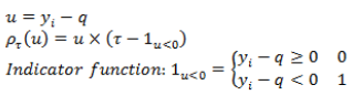
If ordinary least squares regression predicts the mean values of Y ∈ R conditional on the vector x ∈ R^p (or vector of the scores on the predictor variables), quantile regression predicts the values of the median or other quantiles of Y conditional on the vector x. The estimation is performed by minimizing the sum of the absolute deviations. This minimization is usually solved by the simplex method, introduced by Edgeworth (1888) and developed by Barrodale and Roberts (1974). Although other computational options exist, they require large samples, demand more computational resources, and may have more convergence difficulties than the simplex method (Alhamzawi and Ali, 2018; Lustig et al., 1994; Yang et al., 2016).

 

Quantile regression posits the estimation of the quantile of order τ of the variable Y, Q_Y(τ), as a minimization problem (Koenker, 2005).

 

 

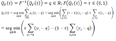
where Q_Y(P) = q = quantile function or inverse of the cumulative distribution function, F_Y(y) = P(Y ≤ y) = τ = cumulative distribution function, τ = cumulative probability or quantile order, q = value of the quantile of order τ of the variable Y, and ρ_τ = loss function of the quantile of order τ of the variable Y.

 

 

Next, the conditional quantile to a linear model based on k predictor variables is defined, and it is proposed to estimate the vector of regression weights through the minimization of the loss function of the conditional quantile (Koenker, 2005).

 

 

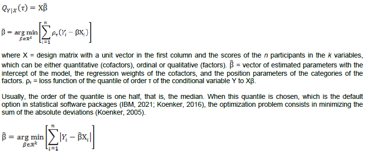
The Statistical Package for Social Sciences (SPSS) can handle multiple cofactors (quantitative variables) and factors (nominal and ordinal variables), taking the last nominal or ordinal category of the factor as the reference category (IBM, 2021; Könker, 2016); likewise, it allows the application of two methods to estimate the parameters: the simplex method (Barrodale and Roberts, 1974; Koenker and d'Orey, 1987) and the Frisch-Newton interior-point method for nonlinear optimization (Frisch, 1956; Lustig et al., 1994). This statistical software chooses the most convenient method as a function of the computational requirements of the task; the simplex method is more suitable for small samples, whereas the Frisch-Newton method is more efficient for large sample sizes (Koenker et al., 2017). By default, the error terms are assumed to be independently and identically distributed, but this option can be changed to covariant and heteroscedastic errors. The scatter plot, where the x-axis represents the observed scores and the y-axis represents the predicted scores, can be examined to find out which assumption fits more to the data set. A funnel-shaped (or an almond-shaped) point cloud indicates the presence of heteroscedastic residuals. In turn, the independence of the errors can be verified through the Wald and Wolfowitz run test (1943) and a graph of the sequence of the residuals, plotted in the order of collection. If the sequence reveals regular patterns, and a residual can be predicted by the previous one or another previous one, it is inferred that there is a serial dependence between the prediction errors.

 

SPSS presents the point estimates, asymptotic standard errors, significance tests with Student's t distribution with n−p degrees of freedom, and 95% confidence intervals for the p parameters (model intercept, regression coefficients corresponding to the cofactors, and position parameters of the categories of the factors), the calculation of the Pseudo R-Squared coefficient suggested by Koenker and Machado (1999), the mean absolute error, the point estimates and 95% confidence intervals for the Y-scores and the residuals. It also computes the variance-covariance matrices and the correlations of the estimated parameters, either through the nonparametric method developed by Bofinger (1975), which is the default method, or through the parametric method proposed by Hall and Sheather (1988).

 

As with other regression methods, it is possible to specify nested effects and interactions between variables (IBM, 2021). Nested effects can be included in the quantile regression model when the values of one variable are only known for specific values of another variable and these two variables do not covary within their full potential range of values. The interaction between variables can be introduced in the model when there is significant and non-linear covariance between two predictor variables (Koenker et al., 2017).

The following is an example of an application of quantile regression. It focuses exclusively on its statistical and analytical characteristics and ignores the theoretical aspects of the field of psychology; therefore, no theoretical framework, hypothesis formulation, or discussion of the data is provided. A relatively small sample size, but appropriate for the technique, was chosen to make the presentation of the analyses more manageable.

 

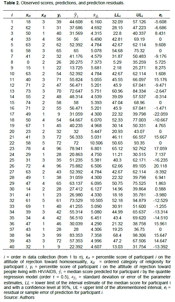
Considering the example a random sample of 40 young adult men (18 to 40 years old) drawn from a population of patients receiving medical care in a medical center located in a city in Mexico. The mean schooling of the participants is 10 years. Religiosity (X₂) is assessed through a closed-ended question. The attitudes toward gay people as well as the attitudes toward people living with HIV/AIDS (Y) are assessed through two self-report scales, namely: the 10-item Scale of Attitude toward Homosexuality (EAH-10) (Moral and Ortega, 2010; Moral and Martínez-Sulvarán, 2012) and the Scale of Attitude toward People Living with HIV/AIDS (Moral and Valle, 2020, 2021). The question regarding religiosity asks about the frequency of attendance at religious services and had five answer options: 1 = never or only in special services related to personal and cultural commitments, 2 = at least once a year motivated by religious faith or religious duty, 3 = at least once a month motivated by religious faith or religious duty, 4 = once or almost once a week, and 5 = at least once a week (Moral, 2010). Scores on the two attitude scales are percentile scores from 1 to 100; in both scales, a higher percentile score evidences a greater level of rejection toward the attitudinal object (that is, a more negative attitude).

 

Now, taking into account the data shown in Table 2, the objective is to estimate a model to predict an attitude of rejection toward people living with HIV/AIDS (quantitative variable measured on an interval scale) as a function of religiosity (variable of ordered categories) and the level of rejection toward gay people (quantitative variable measured on an interval scale) using quantile regression of order τ = 0.5 (predicted median values).

 

Table 1 shows the point and interval estimates of the parameters of the predictive model as well as their asymptotic standard errors and the tests of statistical significance (Student’s t-test with degrees of freedom = n – p = 40 – 6 = 32). Six parameters were estimated (p = 6): the intercept of the model b₀, the regression weight of the cofactor b₁ (attitude toward gay people), and the four position parameters for religiosity b_2|X2=1, b_2|X2=2, b_2|X2=3 y b_2|X2=4 (categories ordered from 1 to 4; category 5 was used as the reference category). The statistical package chose the Barrodale-Roberts simplex method (1974) to estimate these six parameters, being this method the most suitable for the analysis of this small sample (n = 40). It was assumed that the error terms were independently distributed and had homogeneity of variance. In this model, the significant parameters were the intercept, the weight of the attitude toward gay people, and the location parameter of people with very low religiosity (first ordered category); the other three location parameters were not significant (from the second to the fourth ordered category of religiosity).

 

 

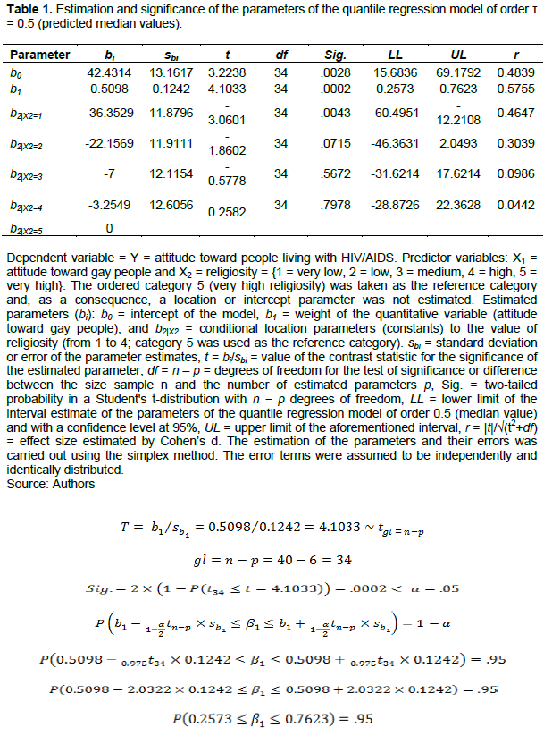
According to Ringquist (2013), for a given regression coefficient whose significance is tested using a Student’s t-test with degrees of freedom df, t = b_j/s_bj ~ t_df, the correlation-based effect size can be estimated through the following statistic: r = |t|/√(t²+df). The effect size with this type of statistic can be interpreted using the cut-off points suggested by Cohen (1988) for the correlation coefficient: 0.1 small, 0.3 medium, 0.5 large, and 0.7 very large. Returning to the data shown in Table 1, the attitude of rejection toward gay people acts as a risk factor for rejection toward people living with HIV/AIDS, b₁ = 0.51, 95% CI [0.26, 0.76], with a large effect size, 0.50 < r = |t|/√(t²+df) = 0.58 < 0.70. A very low level of religiosity, compared to a very high level of religiosity, acts as a protective factor, b_2|X2=1 = −36.35, 95% CI [−60.50, −12.21] and shows a medium effect size, 0.30 < r = |t|/√(t²+df) = 0.47 < 0.50.

 

Table 2 shows the sample data of the 40 participants, as well as the predictions, the error of each prediction, the interval  estimate of the predictions (confidence level at 95%), and the residuals or sample prediction errors.

 

For instance, the first participant obtained an 18th percentile score on the scale that assessed rejection toward gay  people (x₁ = 18),  was  classified as having a medium level of religiosity (x₂ = 3), reached a 39th percentile score in the level of rejection toward people living with HIV/ AIDS (y = 39): the predicted score yielded by the quantile regression model was equal to 44.61 (95% CI [32.09, 57.61]) and the residual was −5.61.

 

 

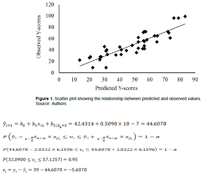
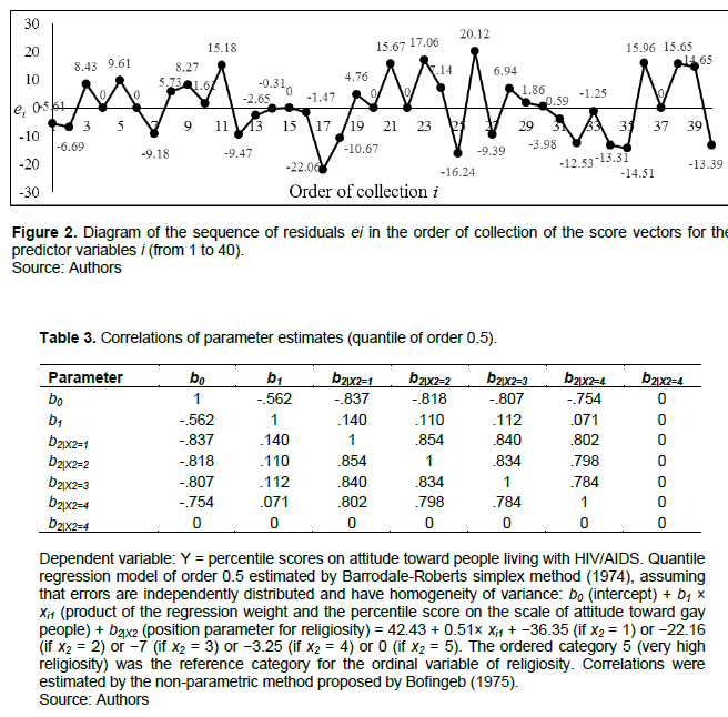
The scatter plot between observed (X-axis) and predicted(Y-axis) Y-scores shows homogeneity in the opening of the point cloud around an ascending straight line (Figure 1). On the other hand, the Wald and Wolfowitz (1943) run test allows us to maintain the null hypothesis of independence of errors. To perform this test, the residuals are arranged in the order of collection of the score vectors (i from 1 to 40); thereafter, the median of residuals is calculated, Mdn(E) = 0, and it is subsequently used as a criterion to dichotomize them: if e_i < Mdn(E), d_i = 0; and if e_i ≥ Mdn(E), d_i = 1. Afterward, the number of residuals lower than the criterion or zeros in D (n₀ = 17) and the number of residues higher than or equal to the criterion or ones in D (n₁ = 23) are counted. Additionally, the runs of zeros and ones in D are calculated (R = 15). Since both n₀ and n₁ are higher than 20, the exact probability is computed. The punctual probability is 0.025, the left-tailed exact probability (R = 15 < Mdn(R) = 20.5) equals to 0.048, and the two-tailed exact probability equals to 0.073, which is a value higher than the conventional level of significance (α = 0.05).  The null hypothesis would also hold with a two-tailed asymptotic probability and a significance level of 0.05: E(R) = 20.55, SD(R) = 3.05, Z = (R−0.5−E(R))/SD(R) = −1.66, Sig. = 2×P(Z ≤ −1.66) = 0.098 > α = 0.05. Likewise, the graph of the sequence of the residuals (in the order of collection of the score vectors for the predictor variables) shows a random order (Figure 2). Consequently, it is appropriate to assume that the residuals are independent and have homogeneity of variance. If these assumptions do not hold, you can change the calculation option in SPSS (IBM, 2021).

 

 

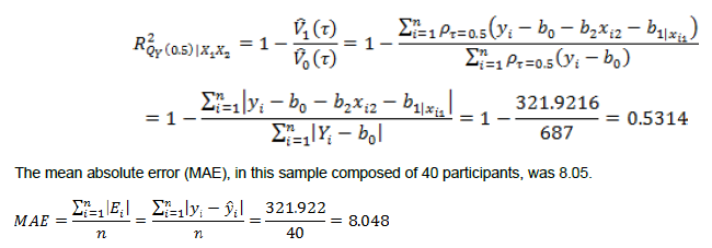
The correlation matrix between the estimated parameters, considering them as random variables, was calculated using the nonparametric method proposed by Bofingeb (1975). This matrix allows us to see that the regression coefficient of the attitude toward gay people (scale parameter) has a trivial correlation with the position parameters of religiosity (from 0.07 to 0.14) and a medium correlation with the intercept of the model (-0.56). The correlations of the position   parameters of religiosity are very high with each other (from 0.78 to 0.85) and with the intercept of the model (from -0.84 to -0.75). The correlations between the parameters of the predictor variables (scale and position) are positive or direct, but the correlations of the predictor variables with the model intercept are negative or inverse (Table 3). This indicates low collinearity between both predictors and linearity between the ordered categories of X₂ (religiosity).

The model showed very good goodness of fit when estimated through the Pseudo R-squared coefficient proposed by Koenker and Machado (1999), which is a local measure of fit that measures the goodness of fit by comparing the sum of the weighted deviations of the final model with the sum of the intercept only model. It only takes into account the fit of the predictions to the observed data, but does not consider the number of variables in the final model or pay attention to parsimony.

 

 

 

Although the deviations from the mean converge toward a Laplace distribution, the average of the absolute deviations does not show such distributional convergence. The one-sample Anderson-Darling test can be used to reject the null hypothesis that posits that the absolute errors follow a Laplace distribution. So, at a significance level of 0.05, the null hypothesis of goodness-of-fit is rejected (AD = 1.139, p = 0.025 < α = 0.05).

 

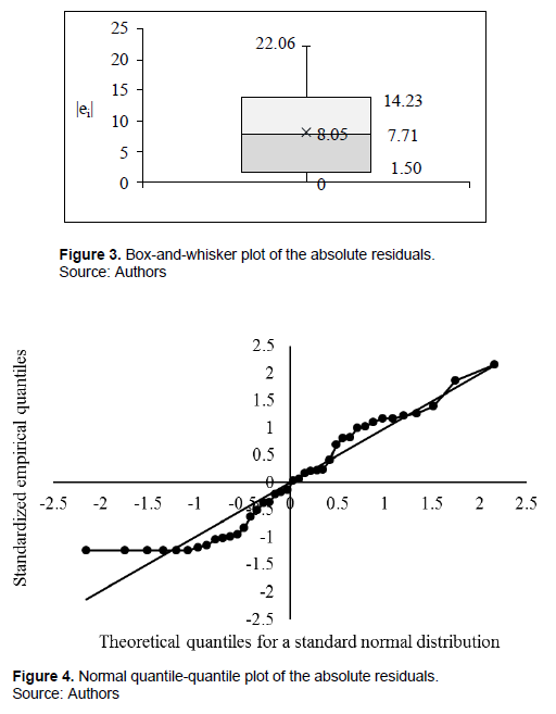
The distribution of absolute residuals is also far from a normal distribution by the Anderson-Darling test (D’Agostino, 1986): A = 0.891, AD = A × (1 + (0.75/n) + (2.25/n²)) = 0.891 × (1 + (0.75/40) + (2.25/402)) = 0.909 > _0.05AD₄₀ = 0.736, p = 0.021 < α = 0.05) and by Shapiro-Wilk W test (Royston, 1992): W = 0.926, p = 0.012). As shown in Figures 3 and 4, the distribution is truncated at its left tail and has a platykurtic profile (Anscombe and Glynn, 1983) test: b₂ = 1.933 < 3, Z = −2.235, two-tailed p = 0.025 < α = 0.05). In the box-and-whisker plot (Figure 3), the lower whisker is cut off at zero and the boxes are wide relative to the whiskers. On the normal quantile- quantile plot centered at 0 (standardized observed and theoretical quantiles), the dotted line flattens out at the lower end in the third quadrant, reflecting a truncated sample (Figure 4). Furthermore, the curve is convex below 0 and tends to be concave above 0 (up to 1.5), which is characteristic of a leptokurtic profile (D’Agostino et al., 1990).

 

Since the distribution is unknown, the confidence interval for the mean absolute error can be estimated by the bias-corrected and accelerated bootstrap interval method (Efron, 1987): PSE = 8.048, bias = −0.0157, SE = 1.037, BCa 95% CI [5.993, 10.099]; number of bootstrap samples: 1000). The 95% confidence interval shows that it is a value significantly different from 0.

 

Binary logistic regression is a technique developed for dichotomized qualitative variables and not for dichotomized quantitative variables (Agresti, 2019). Instead, there is quantile regression, which is a good regression technique for predicting a quantitative variable without distributional requirements of normality or homogeneity of variance in the residuals (Koenker et al., 2017). This technique accepts qualitative, ordinal, and quantitative predictor variables and can even be adapted to correlated residuals (Alhamzawi and Ali, 2018, 2020; IBM, 2021). Moreover, it allows to perform analyses for different quantile orders of the predicted variable; usually, the order is 0.5 (median), but the model can also be estimated for extreme order percentiles, such as 0.25 (lower quartile), 0.75 (upper quartile), 0.10 (first decile) or 0.90 (lower decile); this fact is especially interesting when dealing with heteroscedastic data.

 

The quantile model for the median value would be the counterpart or equivalent to the multiple ordinary least squares linear regression model for the mean value, and the quantile models for the extreme percentiles would be the counterparts or equivalents to binary logistic regression models of the continuous variable dichotomized by the corresponding percentile; nevertheless, quantile regression would be more appropriate to the assumptions made and the measurement scales of the variables included in the model (Waldmann, 2018).

 

Quantile regression is a little-known technique in its theoretical foundations as well as in its aspects of calculation and interpretation in psychological research. However, as can be seen from this article, which uses an example applied to the field of social and health psychology, this technique is clear in its rationale and yields results that are easy to interpret. Therefore, its use is recommended when the data warrant it, which are common situations in research in psychology and related sciences. That is why this regression technique is becoming increasingly used in medical research (Konstantopoulos et al., 2019; Staffa et al., 2019) and is available in statistical packages, such as SPSS (IBM, 2021) and R (Koenker, 2016).

The authors have not declared any conflict of interests.