Full Length Research Paper

ABSTRACT
Increasing greenhouse gas concentrations can cause future changes in the climate system that have a major impact on the hydrologic cycle. To realize and predict future climate parameters, the Atmosphere-Ocean Global Climate Models (AOGCMs) are common employed tools to predict the future changes in climate parameters. The statistical downscaling methods have been applied as a practical tool to bridge the spatial difference between grid-box scale and sub-grid box scale. This paper investigates the capability of Statistical Downscaling Model (SDSM) and Artificial Neural Network (ANN) with different complexities in downscaling and projecting climate variables in the tropical Langat River Basin. These two statistical downscaling models have been calibrated, validated and used to project the possible future scenarios (2030s and 2080s) of meteorological variables, which are the maximum and minimum temperatures as well as precipitation using the CGCM3.1 under A2 emission scenario. The statistical validation of generated precipitation as well as maximum and minimum temperatures on a daily scale illustrated that the SDSM is more accurate than the ANN with different learning rules. On the other hand, the SDSM showed more capability to catch the wet-spell and dry-spell lengths than the ANN model. The calibrated models show higher accuracy in simulating the maximum and minimum temperatures in comparison with the capture of the variability of precipitation. The trend analysis test of generated time series by the SDSM indicates an increasing trend by the 2030s and 2080s at most of the stations.
Key words: Statistical downscaling, multiple linear regression, nonlinear regression, artificial neural network, tropical area, Malaysia.
INTRODUCTION
The studies of climate change impacts on water resources have become an interesting topic since the late twentieth century. The main source of discussion in assessment studies is supported by the outputs from a Global Climate Model (GCM) under different emission scenarios. A GCM is a three-dimensional numerical model of a planetary, ocean and atmosphere that employs many principles of physics, mathematics and fluid mechanics. However, the resolution of GCMs is not high enough to be used directly in a regional study such as a hydrological simulation. In this way, downscaling tools are employed to localize the results of different GCM as an input to hydrological models.
Among the outputs of the GCMs, the temperature and precipitation data were frequently used to force impact model such as hydrological models. In addition, both temperature and precipitation are the main atmospheric variables affected by the Greenhouse Gases (GHG) emissions. For instance, in the Fourth Assessment Report (AR4) of Intergovernmental Panel on Climate Change (IPCC), the climate change effect on fresh water systems is due to increases in temperature and sea level as well as precipitation variability (Fiseha et al., 2012). For the temperature, the report of IPCC AR4 shows the increase of global mean surface temperatures by 0.74ºC over the last 100 years (1906-2005) (Solomon et al., 2007).
The output of GCMs in the simulation of the climate system has coarse resolution that is not enough to match with sub-grid scale features such as topography and landuse. To bridge this gap, downscaling is commonly a method to investigate the impact of climate change on water resources at a regional scale. The basic assumption in downscaling is that the large-scale atmospheric system influences the local scale system considerably, but the inverse effects from regional scales to global scales are insignificant (Fowler et al., 2007; Hewitson and Crane, 1996; Maraun et al., 2010; Teutschbein et al., 2011; Wilby et al., 2004; Xu, 1999).
The existing downscaling methods have two broad categories, namely dynamical downscaling and statistical downscaling, which have been created using atmospheric physics and empirical statistics, respectively. The extensive discussion on these downscaling classes includes theories, application, and advantage and deficiency of them can be found in many previous research works (Hewitson and Crane, 1996;Xu, 1999; Wilby et al., 2004; Fowler et al., 2007; Teutschbein et al., 2011).
Statistical downscaling methods are used by the hydrologist to obtain the local-scale data as an input to the hydrological models. Statistical downscaling approach could be further categorized in weather type, regression method, and weather generator (Wilby et al., 2004). The weather type technique engaged meteorological data to a given weather type in accordance with their similarity concerning synoptic patterns. Regression-based models involve developing a linear or nonlinear empirical relationship between a local climate variable as predictand (e.g. temperature and precipitation) and large-scale GCM parameters as predictors. A Weather Generator (WG) is a stochastic model that can be used to simulate daily weather based on parameters determined by historical records (Wilks and Wilby, 1999). Multiple regression and weather generator methods are more utilized than others, as they are computationally less demanding data, easy to apply, and efficient (Dibike and Coulibaly, 2005; Hashmi et al., 2011; Semenov et al., 1998; Solomon et al., 2007; Tavakolâ€Davani et al., 2013). Moreover, other offered methods, range from Markov Chain (Gregory et al., 1993), and multiple regression (Murphy, 1999)to more complicated hybrid models such as Statistical Downscaling Model (SDSM) (Wilby et al., 1999)and automated regression-based statistical downscaling (Hessami et al., 2008). The comparison of artificial neural network and multiple regression (linear and nonlinear) is the subject of other studies in downscaling climate parameters (Khan et al., 2006; Schoof and Pryor, 2001). However, none of these downscaling methods are robust and precise enough to simulate the diversity in the climate system. Thus, a comparative study of different downscaling models in capturing the temporal characteristics of climate variable would be beneficial (e.g., mean, variance, wet/dry spell length) (Hashmi et al., 2011; Khan et al., 2006; Muluye, 2012). This study investigates and evaluates two statistical downscaling methods in regression category from multiple linear regression (SDSM) to fully nonlinear regression (ANN) in capturing the climatic characteristics in a tropical climate of Malaysia.
Study area
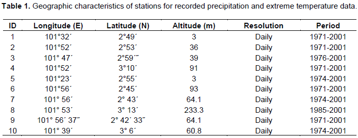
The study area is the Langat River Basin, which is one of the most urbanized catchments in Malaysia, located in the southern parts of Klang Valley in which the capital city of Kuala Lumpur is located (Figure 1). It supplies two third of water required for the state of Selangor for different water usage. This watershed experienced rapid development in urbanization, agriculture, and industrialization. The total area of the Langat River Basin is approximately 2,352 km2. It lies between latitudes 2° 40ËŠ 15ʺ to 3° 16ʹ 15ʺ N and longitudes 101° 17ʹ 20ʺ to 101° 55ʹ 10ʺ E. The northern part of the basin is a mountainous area; while its central and western parts consist of the flat area. The mean areal annual rainfall of the Langat River Basin is 1994 mm, while the highest recorded monthly rainfall is approximately 327 mm in November, and the lowest is 97.6 mm in June. A summary of the geographic characteristics of meteorological stations within the study area is presented in Table 11.
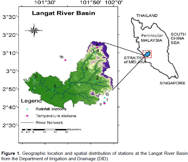
The climatic data used in this study were obtained from the Malaysian Meteorological Department (MMD) and the Department of Irrigation and Drainage (DID). The daily precipitation and maximum and minimum temperatures data of ten stations inside and outside the Langat watershed have recorded of lengths between 16 and 30 years. The geographic location of these stations and river network of study area are shown in Figure 1.
The missing values of precipitation and temperature were calculated using two methods of normal-ratio and Multiple Linear Regression (MLR) between existing and nearby stations with comparable distance and altitude. The NCEP/NCAR reanalysis dataset and large-scale predictors of the third generation of Coupled Global Climate Model (CGCM3.1) version T47 for baseline period as well as Special Report on Emission Scenarios (SRES) A2 were used to develop the downscaling model and projection of daily precipitation and maximum and minimum temperatures for the two future periods. On the list of SRES scenarios, A2 is known among the most severe scenario, projecting high emissions in the future (Nakićenović et al., 2000).
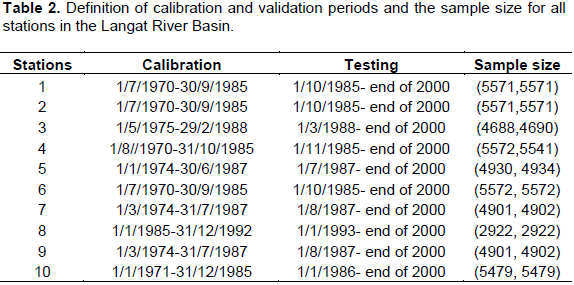
The closest grid cell for the study area has coordinates of 1.86°N and 101.25°E (X=28 and Y=24). In this research, the current climate as the base line period was set for the starting date of recording until the end of the year 2000 (Table 2). Two projection time slices, namely 2020-2049 (2030s) and 2070-2099 (2080s) exist, which allow the assessment of climate change impacts on water resource in the watershed.
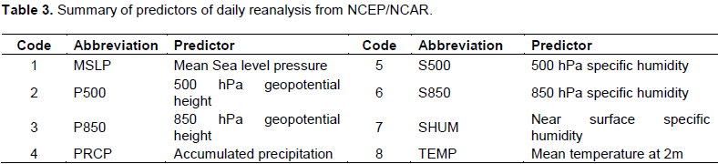
While the original predictor dataset of NCEP/NCAR contained 26 daily predictors (describing atmospheric circulation, thickness and moisture content at the surface, geopotential heights at 850 and 500 hPa), the candidate predictors are only eight predictors in Malaysia. This limitation is for an area near the equator (this study area) where Coriolis forces tend to be zero (Predictors, 2008). The candidate lists of large-scale predictor variables from NCEP/NCAR and CGCM3.1 used in downscaling the climate variables are presented in Table 3. The values of predictors were normalized by their respective mean and standard deviation.
METHODOLOGY
Downscaling model description and setup
In this study, two statistical downscaling models including Statistical Downscaling Model (SDSM), and Artificial Neural Network (ANN) were used in downscaling the local hydrological variables on a daily scale (precipitation, maximum and minimum temperatures) using the large-scale predictors. Seven stations were selected for precipitation, while three stations were selected for temperature (TMax and TMin). Some primary process steps such as quality control and screening the predictors are taken to create a common dataset for these statistical downscaling methods. In this study, the fourth root transformation has been conducted for precipitation, which is usually skewed climatic variable as preprocessing for the application of the SDSM model (Chen et al., 2011).
Statistical downscaling model
The Statistical Downscaling Model (SDSM) uses of a hybrid of stochastic weather generator and multiple linear regression techniques in downscaling the climate variables. This technique permits the spatial downscaling through daily predictor-predictand relationship using multiple linear regressions and generates predictands which represent the local weather. This statistical downscaing model is a combination of a stochastic weather generator technique and a transfer function model (Wilby et al., 2002) which needs two types of daily data. the local predictands of interest (e.g. temperature and precipitation) is the first and the data of large-scale predictors (NCEP and GCM) of a grid box closest to the study area is the second type of data sets (Wilby et al., 2002). Wilby et al. (2002)described seven major steps for developing the best execution of the multiple linear regression equation for the downscaling process, including quality control and data transformation; screening of predictor variables; model calibration weather generation (using observed predictors); statistical analyses graphing model output and finally scenario generation (using climate model predictors). Unlike the simple multiple linear regression, the temperature and precipitation variables are modeled as an unconditional and conditional process, respectively. In the conditional method, the large-scale circulation behavior as well as atmospheric moisture parameter is utilized to linearly condition local-scale weather generator variables like precipitation occurrence and also the intensity (Wilby et al., 2002). Then, the generated daily time period was adjusted for its mean and variance by using bias correction and variance inflation factors, respectively, with regard to reach a better agreement with observed data, which are set to 12 and 1, respectively, in the calibration period as proposed by Hessami et al. (2008).
Artificial neural network
The second downscaling method is the Artificial Neural Network (ANN) under the Multilayer Perceptron (MLP) architecture with variation of learning algorithms, transfer functions, and number of neurons. The ANN is a nonlinear regression type which the network learned by supervised and unsupervised learning to create a developed relationship between a few selected large-scale atmospheric predictors and basin scale meteorological predictands.
The MLP is one of the most popular neural network, which consists of three layers of neurons namely, input, hidden and output layer. The information flows in the forward direction and network trained using a back propagation learning algorithm to minimize the least square error (LSE) between realized and target outputs. As weights in MLP computed by a developed back-propagation learning algorithm, these networks are the most popular among researcher and users of ANNs (Jain et al., 1996). The Multi-layer perceptron with one hidden layer and three learning algorithms include Momentum (M) (Harpham and Wilby, 2005), Levenberg-Marquardt (LM) (Govindaraju and Rao, 2010), and Conjugate Gradient (CG) learnings (Charalambous, 1992) which were investigated for downscaling the precipitation, maximum and minimum temperatures at 10 stations. The transfer functions in hidden layer were Sigmoid (Sig) and Hyperbolic Tangent (HT) and also linear transfer function in the output layer. The numbers of hidden layer neurons were found through simple trial-and-error method in all applications. Then, the performances of different networks were examined using correlation coefficient (R), and MAE.
Validation of models
The parameters established during the calibration process that explain the statistical agreement between observed and simulated data were then used for the model validation and for daily and monthly time scales.
The performance of downscaling models in generating the mean daily precipitation, mean dry spell and wet spell length for precipitation in a month and mean daily and variance for temperature in a month were examined using the Standard Error (SE), Mean Absolute Error (MAE), and Root Mean Square Error (RMSE) as follows:
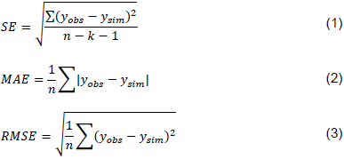
Where, yobs is the observed data, ysim is the simulated value, k is the number of independent variables, and n is the number of recorded data in the validation dataset. The y refers to daily maximum temperature, minimum temperature and precipitation at each station. In this study, a dry day is defined as a day with an amount of less than 1 mm precipitation during a day (Deni et al., 2010).
Uncertainty analysis
In the statistical downscaling, confidence intervals in the estimates of means and variances provide special view about uncertainty in the estimates of mean and variances (Khan et al., 2006). In the current study, the most commonly used non-parametric technique, bootstrapping has been applied to obtain the confidence intervals of means and variances. The main part of bootstrapping is to resample a large number of new data sets with replacement from the original data set. The algorithm for uncertainty analysis in this study includes the following steps:
1. Draw a new sample of size n with replacement from the original sample.
2. Compute the mean or variance of the new sample.
3. Repeat steps 1 and 2, 1000 times, and calculate the mean and variance.
4. Plot the distribution of these 1000 sample means or variances.
5. Compute the 95% confidence interval for the mean or variances by finding the 2.5th and 97.5th percentiles of this constructed distribution.
RESULTS AND DISCUSSION
Selection of Predictors
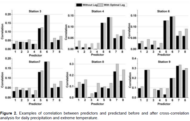
The selection of predictors mainly ascertains the character of the downscaled climate scenario. As the correlation analysis between the predictands of the Langat River Basin and the NCEP/NCAR re-analysis predictors was discovered to have extremely poor results, an offline statistical analysis was carried out to improve the correlations between predictand and predictors (Hashmi et al., 2011). A Cross Correlation Analysis (CCA) between each pair of predictands and the NCEP/NCAR predictors is an attempt in this regard to find the optimum lags, which correspond with maximum correlation between each pair of predictand-predictors.
The correlation amounts before and after CCA at six out of 10 stations are shown in Figure 2 as an example. While for many of the NCEP/NCAR predictors at the stations, the CCA improved the correlation between the large-scale predictors and local-scale predictand, few of the NCEP/NCAR predictors did not show any lag for the improvement of the correlation. The examination of the results of the CCA indicates that improvements in the predictors include MSLP, P500, and P850, which were more than that for S850, SHUM, and TEMP. The comparison between predictand-predictors correlation shows that the correlation coefficient for maximum and minimum temperatures are higher than that for daily precipitation as a predictand. This lagged NCEP/NCAR predictors and the local precipitation as well as maximum and minimum temperatures are then employed to screen the predictors as a process in the calibration of the statistical downscaling models.
The stepwise regression with both directions (backward and forward) was adapted to screen the predictors and select the best combination of them by reaching the smallest Akaike Information Criterion (AIC) (Hessami et al., 2008; Tavakolâ€Davani et al., 2013). Table 4 shows the identified significant NCEP/NCAR predictors for predictand and stations at the significant level of p <0.001 under consideration.
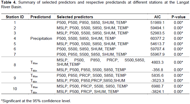
From the selected predictors in Table 3, it was discovered that the local variables were controlled by non-atmospheric parameters. For instance, both of temperature and precipitation are sensitive to pressure fields at geopotential heights of 500 hPa, and near surface specific humidity.
While, the Mean Sea Level Pressure (MSLP) is a measure control variable for temperature, it was not a significant predictor for precipitation in all sites. The mean temperature at 2 m height (TEMP) controls both the maximum and minimum temperatures and precipitation observed at each station except minimum temperature at Station 9.
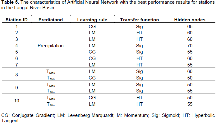
The selected predictors at all stations were used for the calibration and validation of different downscaling models including SDSM version 4.2.9 (Wilby et al., 2002), and artificial neural network with different structures. The observed historical dataset until the year 2001 was split into two equal parts of the calibration and validation processes of the downscaling methods as defined in Table 2. The calibration of two statistical downscaling approaches was carried out for every single site during the calibration period and validated through the data outside the calibration period.
Comparisons of model performance
Two downscaling approaches were examined in simulating the predictand time series during the validation period (independent data set) as described in Table 2 and Table 5 at all stations in the Langat River Basin. The performance results of the validation criteria include the SE, RMSE, and MAE of the satisfactory calibrated downscaling models, which are presented in Table6. The results of the validation analysis indicated that the SDSM technique performed lower value of error (SE, RMSE, and MAE) in reproducing the observed time series of temperature and precipitation than the ANN model. Therefore, the SDSM model was more efficient in reproducing the inter-annual variability (less error value) of the mean daily precipitation and daily maximum and minimum temperatures compared to the other model (Sachindra et al., 2013). The result also showed less error values in downscaling the maximum and minimum temperatures than the precipitation by the two models. It is noted that the lower error (SE, RMSE, and MAE) values during the calibration and validation lead to the better performance of the model.
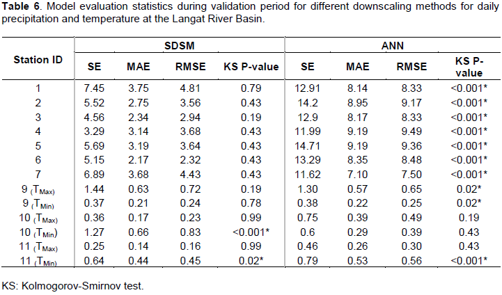
The results of the Kolmogorov-Smirnov (KS) test in Table6 indicated no significant difference between the produced mean values of precipitation by SDSM and the observed values at the 95% confidence level. The only acceptable modeling by the ANN was produced at Station 10 in downscaling the TMin during the validation period. The results of KS test also showed that none of these downscaling models were capable to reproduce the mean monthly TMin at Station 11.
The statistical characteristics of daily precipitation time series are important for the future projection of downscaling models.
Table 7 illustrates the statistical characteristics of downscaled precipitation including the ratio of dry days, which were bracketed by downscaling models as well as mean and standard deviation (SD) in the validation period at the stations of the Langat River Basin. In addition to the better accuracy of the SDSM in simulating the historical observed time series, its skill in reproducing the number of dry days (P <1 mm) and SD of time series was more acceptable. In comparison, in these two downscaling techniques, it seems that the SDSM is more capable in simulating the number of dry day, wet day and SD of rainfall data.
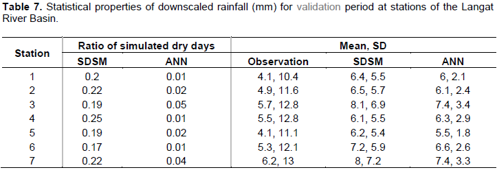
It is not unusual to receive negative precipitation value forecasts from the ANN models (Muluye, 2012). From this point of view, while the SDSM model was smart in generating non-negative values, the ANN technique performed negative values in daily rainfall during the validation period, respectively.
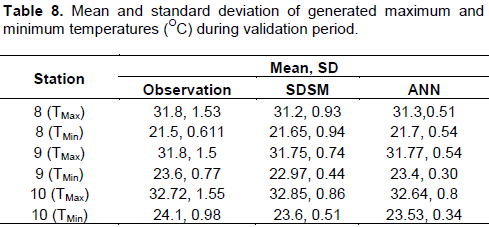
For the maximum and minimum temperatures, while, the performance of the ANN method was acceptable in reproducing the mean observed values, the SDSM model produces qualified time series in reproducing the standard deviation of the observation (Table 8).
As the average length of monthly dry-spell and wet-spell length and variance of temperature are essential analysis measures, which are widely used to evaluate the reliability of the downscaled precipitation. In addition to considering the verification of mean monthly precipitation, a comparative plot of observed and downscaled variables is shown in Figure 3 as an example of all stations in the Langat River Basin. These results showed that in comparison to the generated downscaled time series for precipitation and temperature and their observed counterparts, the SDSM model generated comparable results for mean, dry spell, wet spell length, and variance of maximum and minimum temperatures at all sites in the Langat River Basin. A dry and wet spell length was presented as the maximum number of consecutive dry and wet days in a month, respectively, which is computed for different downscaling models in the validation period as well as future projection periods (2030s and 2080s). While, the ANN model underestimated the mean daily rainfall, their performances were, however, reasonably better in simulating the monthly mean of the minimum and maximum temperatures.
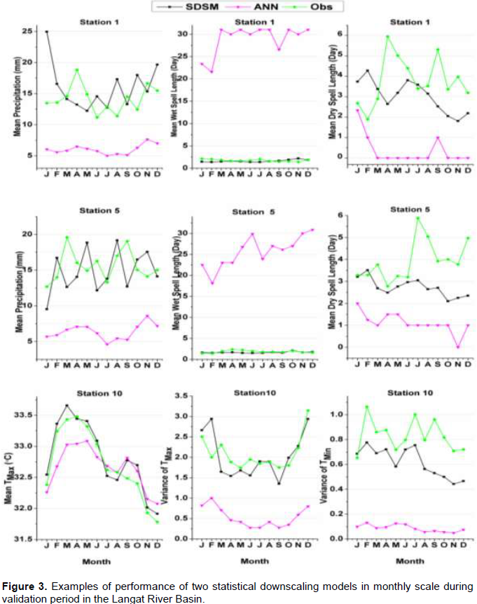
The performance of the ANN models in downscaling the mean, dry spell, and wet spell length behavior shows that these models are poor in generating the precipitation statistics that have been reported by Khan et al. (2006). In other words, these models overestimate the wet spell length, and underestimate the mean monthly precipitation and dry spell length in comparison to the SDSM technique (Figure 3). The poor performance may be due to the fact that these models tend to simulate the low value of precipitation even in dry days. In addition, the reasonable performance of the SDSM may be due to the use of conditional process in modeling the precipitation in time series. Therefore, the complexity of the regression models (ANN) alone is not sufficient in simulating the time series of climate parameters specially rainfall. Finally, the two downscaling models were applied to generate the future scenario (2030s and 2080s) of the rainfall, maximum and minimum temperatures as regional climatic variables at all stations.
Generation of future climate scenarios
Here, the future climate scenarios are generated for daily precipitation; mean daily minimum and maximum temperatures by two calibrated downscaling models including the SDSM, and ANN models in single site approach. In all of these downscaling models, the A2 emission scenario from CGCM3.1 T47 was used to produce the future climate scenario for 2030s (2020-2049) and 2080s (2070-2099) periods.
Projected daily precipitation
The precipitation daily scenarios for the two future periods of 2030s and 2080s were generated at all stations in the Langat River Basin. The results of monthly mean precipitation and temperature, dry spell and wet spell length of the generated scenario of the climate variables in the 2030s and baseline periods are shown in Figure 4.
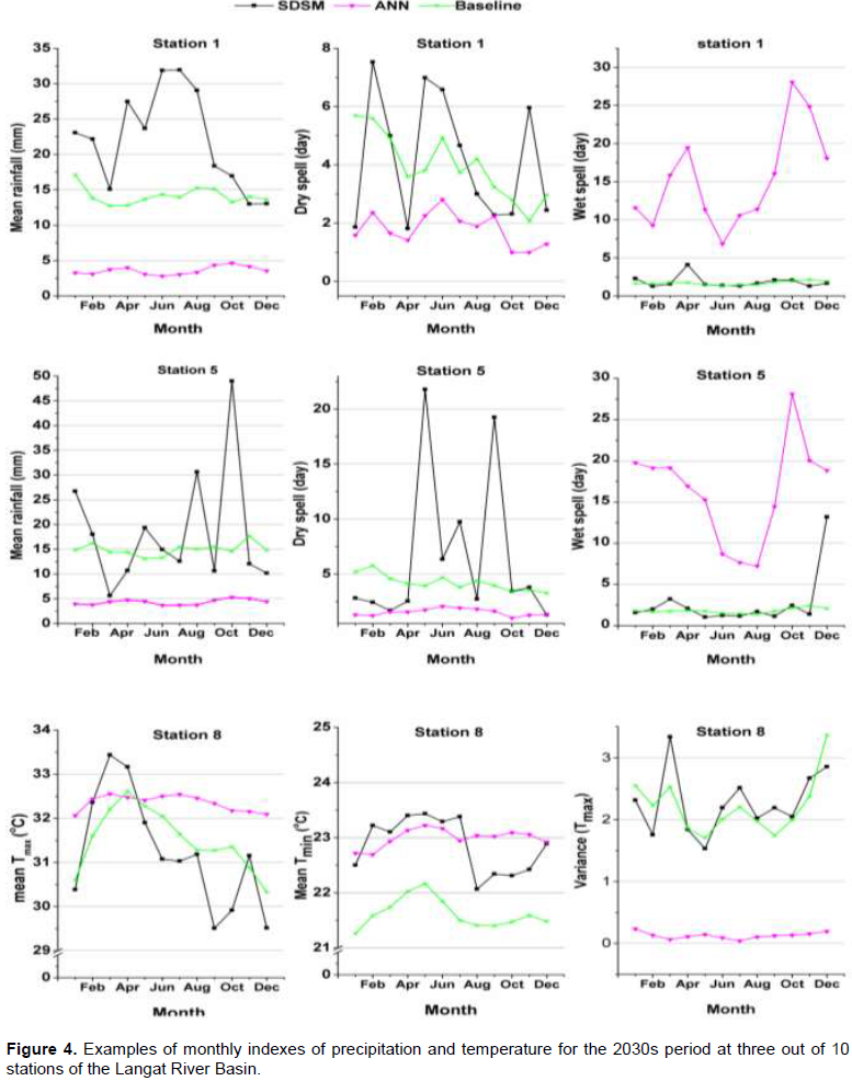
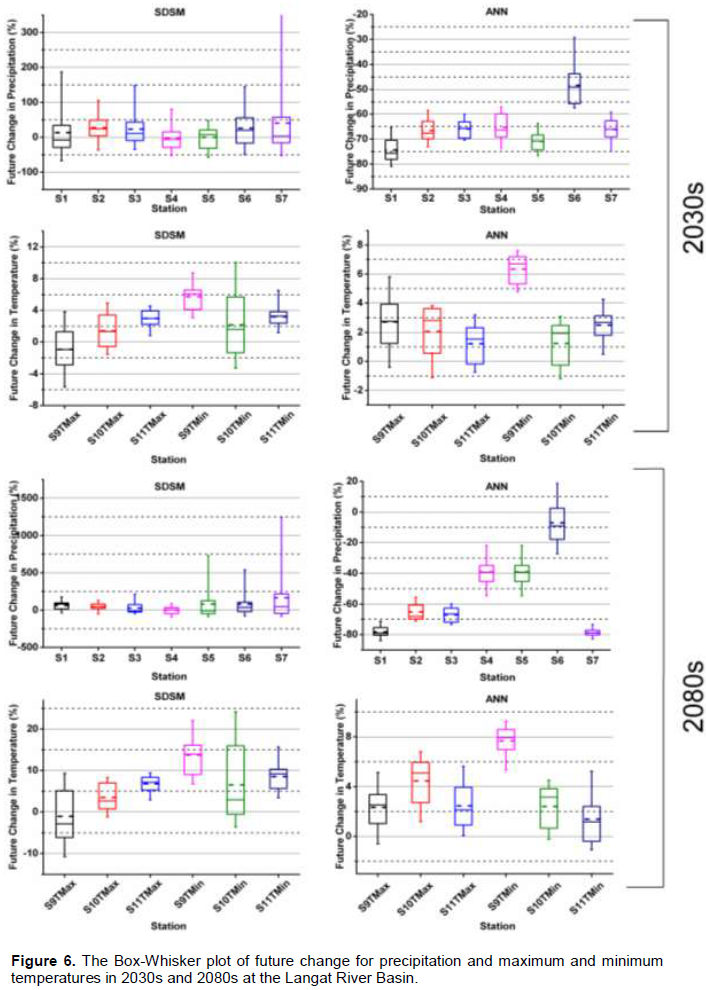
It is indicated that while the mean monthly rainfall generated by SDSM technique, predicted an increase in the mean monthly rainfall at most of the stations, the other downscaling technique, anticipated a decrease in this value in two future projected periods compared to the current period (Figure 6). The average percentage of the change of mean monthly precipitation in the 2030s predicted by the SDSM, and ANN models at different stations varies between 34 to 113, and -70.9 to -48.4%, respectively. Therefore, the SDSM and ANN models predicted increasing and decreasing changes in mean monthly precipitation for the 2030s, respectively. The changes predicted by these models at different stations by the 2080s period are in the ranges between 25 and 254 and -78.7 and -7.1%, respectively. As observed, the ranges of the variation of mean monthly rainfall at different stations by 2080s period are wider than those in the 2030s. The results of the box-Whisker statistics are shown in Figure conform to this reality. The results of the SDSM show an increase in the values of rainfall through the southwest monsoon rainfall by 2030s compared to the baseline period. The comparative plots of monthly dry spell and wet spell lengths between the current period and downscaled daily precipitation in the 2030s period using two downscaling methods are shown in Figure 4 for Stations 1 and 4 as an example.
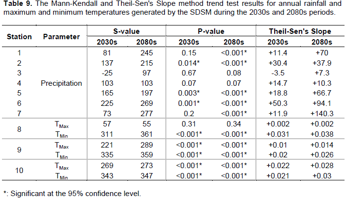
The results of the trend analysis using the Mann-Kendall and Theil-Sen's Slope method for annual rainfall in two future periods are shown in Table 9. It illustrates that significant increasing trends exist in two future periods. The rate of changes in significant trends for the 2080s period was higher than that in the 2030s. The projected annual rainfall for two future periods at Stations 2 and 3 did not indicate any significant trend for the two future periods at the 5% significance level.
It was found that the ANN downscaling model anticipated a decrease in dry spell and an increase in wet spell lengths in the 2030s and 2080s periods. Thus, this model predicted an increase in the number of rainy days and a decrease in the daily rainfall amount for this river basin in the 2030s and 2080s compared to the current period. As discussed in the calibration section, the ANN model showed poor estimation of dry and rainy days, therefore, its projection of dry spell and wet spell lengths for future periods are weak in comparison to the projection of the SDSM. This is the reason that the rate of changes, which predicted the ANN in the 2030s and 2080s compared to the current period, is unrealistic and extremely high. On the other hand, the SDSM simulations of these statistics fluctuate in different months and stations.
The analysis of generated precipitation time series by these models indicated that the predicted trend, which was generated for the 2030s, also continues in the 2080s period. The rate of change for dry spell and wet spell lengths by the SDSM is less than that of the other downscaling model.
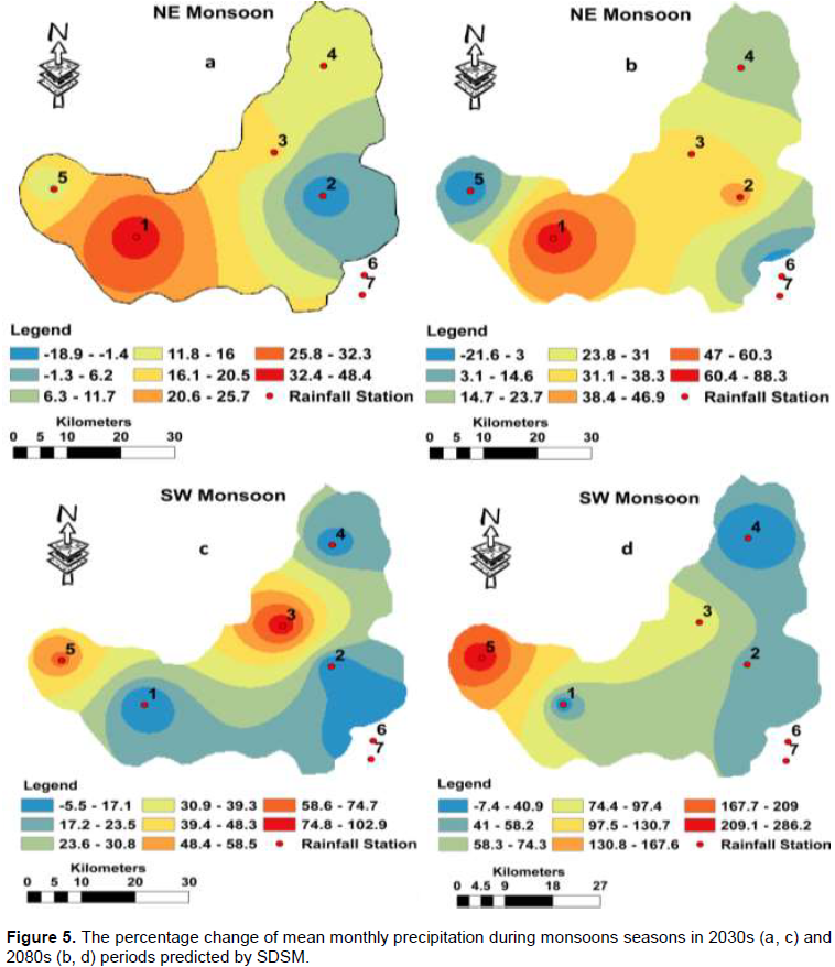
As mentioned before, the SDSM generated more reliable results during the validation period. Therefore, the maps of change percentage during the two monsoons seasons for the two future periods were created using the IDW technique for the study area (Figure 5). As can be seen, the flat area of the basin shows more change than the mountainous area in the future periods. In addition, the area close to cities illustrated higher percentage of change than area with forest land cover.
Maximum temperature
The projected mean maximum daily temperature in the month during the 2030s and 2080s under the A2 emission scenario (Figure 4 and Figure 6) were generated using two statistical downscaling methods. The downscaling results of the models indicated that most of sites in the river basin experience an increase in TMax during two future periods. The rate of change was positive in the southwest monsoon months (May to August) and slight declines were there in the northeast monsoon months (November to February). It can be seen that the results of the two models are consistent in predicting the positive and negative changes of TMax. In general, the SDSM, and ANN models predicted an increase in monthly TMax by 0.37 and 0.62°C, respectively. Therefore, the SDSM projection illustrated smaller changes in TMax by the 2080s period in comparison with the ANN model. The rate of future change produced by the SDSM, predicted lower change at Station 8 in comparison with other stations (Figure 6). As shown in Figure 1, this station is located in a mountainous area and forest land cover. The variance of generated daily maximum temperature during the first future period under the A2 emission scenario at Station 8 is illustrated in Figure 4. It shows that the variance of generated time series by the ANN model has less fluctuation over month during the 2030s period related to the SDSM. The SDSM model attempts to replicate the variance of maximum temperature in the current period for the 2030s and 2080s periods as the variance inflation adjustment in the calibration process of SDSM forced the model to follow the observed data (Wilby et al., 2002).
The results of trend analysis indicated that, while there was a significant trend in the predicted annual TMax at Stations 9, the trend test did not detect any significant trend for two future periods at the 95% confidence level. The rate of changes in the significant trends obtained by Theil-Sen's test in the 2080s period was larger than that in the 2030s period.
Minimum temperature
The scenario outcome of the two downscaling models has not shown a unique increasing or decreasing pattern in the minimum temperature at the Langat River Basin. While the SDSM model expects a decrease in the mean values of TMin for the southwest monsoon months, the other downscaling model predicted increasing changes by the 2030s and 2080s periods. Almost both of the generated downscaling time series under the A2 emission scenario showed the highest rate of change percentage by the 2030s and 2080s at Station 8, where located in a mountainous area in comparison with the stations in flat areas (Figure 1).
The Box-Whisker of downscaled minimum temperature at the stations of this basin explored more variability in the generated minimum temperature than the maximum temperature time series. The downscaling results of TMin by the SDSM, and ANN models predicted a mean increase of 0.83 and 0.75°C at the stations of this basin by the 2030s, respectively. These rates were 2.2 and 0.84°C for the 2080s period. As illustrated, both of the models forecasted an increase in TMin in both of the two future periods.
The downscaled minimum temperature projected by the ANN model indicated the lower rate of variance at the stations of the Langat River Basin by 2030s in comparison with the SDSM. These results also indicated the mean variance of TMin by 1.0, and 0.16 in projected time series generated by the SDSM, and ANN models for the 2080s period. The Mann-Kendall test analysis detected an increasing trend in the annual TMin generated by The SDSM for the two future periods at all stations of the Langat River Basin. The Theil-Sen's Slope method obtained higher increasing rates in the annual TMin for the 2080s than the 2030s period. The difference of change slopes in the 2030s and 2080s in predicted annual rainfall was higher than that for the annual maximum and minimum temperatures (Table 9).
CONCLUSIONS
This study examined the effects of the complexity of regression models in downscaling the climate variables in a tropical watershed in Malaysia. The performance of a multiple linear regression, called SDSM, and non-linear regression, called artificial neural network with three significant learning rules were evaluated in simulating presence and projecting the two future periods (2020-2049, 2070-2099) of daily precipitation, maximum and minimum temperatures under the A2 emission scenario using CGCM3.1. The three learning algorithms were Momentum, Levenberg-Marquardt, and Conjugate Gradient. The daily precipitation, maximum and minimum temperatures from the beginning of recording period were used as weather inputs to the downscaling model. These two downscaling models were calibrated and validated using large-scale predictors NCEP/NCAR reanalysis data and regional climate variables. The comparison of generated time series illustrated that the SDSM was more accurate than the ANN model. While the SDSM showed more ability to catch the wet-spell and dry-spell length, the other model overestimated the wet-spell length, and underestimated the mean monthly precipitation and dry-spell length. The calibrated models for precipitation and temperature devised here performed relatively better in simulating the temperature, but relatively poor to capture the variability of precipitation.
The SDSM predicted an increase in the mean monthly precipitation, while, the other model anticipated a decline in this value by the 2030s period. The range of these rates was wider for the 2080s than the 2030s period. The results of the SDSM showed an increasing change in rainfall through the southwest monsoon season rainfall in the 2030s compared to the baseline period. The time series of daily precipitation in the two future periods generated by the ANN downscaling model indicated a decrease in the dry spell and an increase in the wet spell length in the 2030s and the 2080s, which did not conform to the SDSM results. The downscaling models indicated that most of the sites in the river basin experience an increase for TMax during the two future periods, but the rate of change is more during the southwest monsoon month (May to August) and slightly less during the northeast monsoon (November to February). Therefore, warmer weather conditions in the two future periods were predicted by the downscaling models. The results of the SDSM and other downscaling model found different expectations in the prediction of TMin for the southwest monsoon season months.
The SDSM predicted a decrease and the other downscaling model predicted an increasing trend by the 2030s and the 2080s periods. Almost all the generated downscaling time series under the A2 scenario showed the highest rate of change percentage by the 2030s and the 2080s at Station 8, which located in a mountainous area in comparison with the stations in flat areas.
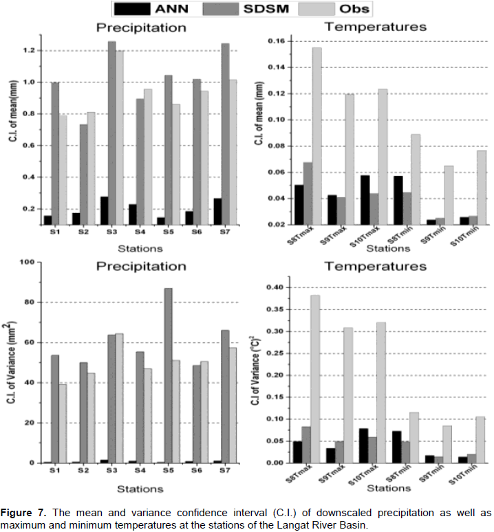
The uncertainty in the estimation of means of the observed and downscaled daily precipitation as well as daily maximum and minimum temperatures has been measured by estimating confidence intervals about means and variance at different stations (Figure7). The uncertainty analysis of the estimates of mean and variance is performed by calculating the 95% non-parametric bootstrap confidence intervals of these variables using the available data (Error! Reference source not found.2). The uncertainty of mean and variance of the observed daily precipitation as well as maximum and minimum temperatures have been compared with the uncertainty of the downscaled mean and variance daily precipitation and maximum and minimum temperatures. The graphical plots of those uncertainty estimates are shown in Figure7. In the case of daily precipitation downscaling, This figure indicates that the ANN model variability is not close enough with the observed variability but the SDSM variability are closer to the observed variability at all stations. The uncertainty of ANN and SDSM models indicated that the variability between the observed and simulated daily maximum and minimum temperatures cannot be considered equal at most of stations.
CONFLICT OF INTERESTS
The authors have not declared any conflict of interests.
ACKNOWLEDGEMENTS
The authors would like to thank the Department of Irrigation and Drainage (DID) and the Malaysian Meteorological Department (MMD), both under the Ministry of Natural Resources and Environment Malaysia (NRE), for providing the data and technical support. The authors would also like to thank the Ministry of Science, Technology and Innovation (MOSTI) sincerely for the financial support provided for the project.
REFERENCES
|
Charalambous C (1992). Conjugate gradient algorithm for efficient training of artificial neural networks. Circuits Devices Syst. 139(3):301-301. |
|
|
Chen J, Brissette FP, Leconte R (2011). Uncertainty of downscaling method in quantifying the impact of climate change on hydrology. J. hydrol. 401(3):190-202. |
|
|
Deni SM, Jemain AA, Ibrahim K (2010). The best probability models for dry and wet spells in Peninsular Malaysia during monsoon seasons. Int. J. Climatol. 30(8):1194-1205. |
|
|
Dibike YB, Coulibaly P (2005). Hydrologic impact of climate change in the Saguenay watershed: comparison of downscaling methods and hydrologic models. J. Hydrol. 307(1):145-163. |
|
|
Fowler H, Blenkinsop S, Tebaldi C (2007). Linking climate change modelling to impacts studies: recent advances in downscaling techniques for hydrological modelling. Int. J. Climatol. 27(12):1547-1578. |
|
|
Govindaraju RS, Rao AR (2010). Artificial neural networks in hydrology: Springer Publishing Company. |
|
|
Gregory J, Wigley T, Jones P (1993). Application of Markov models to area-average daily precipitation series and interannual variability in seasonal totals. Clim. dyn. 8(6):299-310. |
|
|
Harpham C, Wilby RL (2005). Multi-site downscaling of heavy daily precipitation occurrence and amounts. J. Hydrol. 312(1-4):235-255. |
|
|
Hashmi MZ, Shamseldin AY, Melville BW (2011). Comparison of SDSM and LARS-WG for simulation and downscaling of extreme precipitation events in a watershed. Stoch. Environ. Res. Risk Assess. 25(4):475-484. |
|
|
Hessami M, Gachon P, Ouarda TB, St-Hilaire A (2008). Automated regression-based statistical downscaling tool. Environ. Model. Softw. 23(6):813-834. |
|
|
Hewitson B, Crane R (1996). Climate downscaling: techniques and application. Clim. Res. 7(2):85-95. |
|
|
Jain AK, Mao J, Mohiuddin KM (1996). Artificial neural networks: A tutorial. Computer 29(3):31-44. |
|
|
Khan MS, Coulibaly P, Dibike Y (2006). Uncertainty analysis of statistical downscaling methods. J. Hydrol. 319(1-4):357-382. |
|
|
Maraun D, Wetterhall F, Ireson A, Chandler R, Kendon E, Widmann M, Themeßl M (2010). Precipitation downscaling under climate change: recent developments to bridge the gap between dynamical models and the end user. Rev. Geophys. 48(3). |
|
|
Muluye GY (2012). Comparison of statistical methods for downscaling daily precipitation. J. Hydroinformatics 14(4):1006-1006. |
|
|
Murphy J (1999). An evaluation of statistical and dynamical techniques for downscaling local climate. J. Clim. 12(8):2256-2284. |
|
|
Nakićenović N, Alcamo J, Davis G, de Vries B, Fenhann J, Gaffin S, Grübler A (2000). IPCC Special Report on Emissions Scenarios (SRES), Working Group III, Intergovernmental Panel on Climate Change (IPCC): Cambridge University Press, Cambridge. |
|
|
Predictors DC (2008). Sets of predictor variables derived from CGCM3 T47 and NCEP. NCAR Reanalysis, version, 1. |
|
|
Sachindra D, Huang F, Barton A, Perera B (2013). Least square support vector and multiâ€linear regression for statistically downscaling general circulation model outputs to catchment streamflows. Int. J. Climatol. 33(5):1087-1106. |
|
|
Schoof JT, Pryor S (2001). Downscaling temperature and precipitation: A comparison of regressionâ€based methods and artificial neural networks. Int. J. Climatol. 21(7):773-790. |
|
|
Semenov MA, Brooks RJ, Barrow EM, Richardson CW (1998). Comparison of the WGEN and LARS-WG stochastic weather generators for diverse climates. Clim. Res. 10(2):95-107. |
|
|
Solomon S, Qin D, Manning M, Chen Z, Marquis M, Averyt K, Miller H (2007). Summary for Policymakers. Climate Change 2007: The Physical Science Basis. Contribution of Working Group I to the Fourth Assessment Report of the Intergovernmental Panel on Climate Change: Cambridge University Press, Cambridge, United Kingdom and New York, NY, USA. |
|
|
Tavakolâ€Davani H, Nasseri M, Zahraie B (2013). Improved statistical downscaling of daily precipitation using SDSM platform and dataâ€mining methods. Int. J. Climatol. 33(11):2561-2578. |
|
|
Teutschbein C, Wetterhall F, Seibert J (2011). Evaluation of different downscaling techniques for hydrological climate-change impact studies at the catchment scale. Clim. Dyn. 37(9-10):2087-2105. |
|
|
Wilby R, Charles S, Zorita E, Timbal B, Whetton P, Mearns L (2004). Guidelines for use of climate scenarios developed from statistical downscaling methods. |
|
|
Wilby R, Dawson CW, Barrow EM (2002). SDSM—a decision support tool for the assessment of regional climate change impacts. Environ. Model. Softw. 17(2):145-157. |
|
|
Wilby R, Hay LE, Leavesley GH (1999). A comparison of downscaled and raw GCM output: implications for climate change scenarios in the San Juan River basin, Colorado. J. Hydrol. 225(1):67-91. |
|
|
Wilks DS, Wilby RL (1999). The weather generation game: a review of stochastic weather models. Progress Phys. Geogr. 23(3):329-357. |
|
|
Xu C-Y (1999). From GCMs to river flow: a review of downscaling methods and hydrologic modelling approaches. Progress Phys. Geogr. 23(2):229-249. |
|
Copyright © 2024 Author(s) retain the copyright of this article.
This article is published under the terms of the Creative Commons Attribution License 4.0


