ABSTRACT
The performances of five empirical models, namely: Hargreaves-Samani, Makkink1 (1957), Makkink2 (1984), Priestley-Taylor and FAO 56-PM in estimating reference evapotranspiration (REF-ET) were separately compared with Epan data and FAO 56-PM, respectively. Based on statistical analysis, Hargreaves-Samani method compared best with daily and monthly Epan data, while Makkik2 (1984) ranked first with FAO 56-PM. In terms of regression analysis, Priestley-Taylor performed best with daily FAO 56-PM method while Hargreaves-Samani ranked first with daily Epan data. Hargreaves-Samani also correlated best with mean monthly Epan data. The quantitative evaluation of cumulative daily and monthly reference-evapotranspiration (RET-ET) values showed that Makkink (1984) produced the least overestimation and percent relative error against FAO 56-PM while Hargreaves-Samani performed best with Epan data with the least overestimation and percent relative error. In terms of cumulative monthly ETo totals for the farming season (Dec-April) over the study period, Hargreaves-Samani ranked best with Epan data with the least overestimation and percent relative error while Priestley–Taylor ranked best with FAO 56-PM producing the least overestimation. Overall, Hargreaves-Samani with its original coefficient was adjudged best, capable of approximating FAO 56-PM and Epan data in the Lower Niger River Basin, followed by Makkink (1984) and Priestley-Taylor. Penman-Monteith estimates were used to develop monthly correction factors for adjusting Empirical models for their potential use in Lower Niger Basin. A comparative study such as this has not been undertaken in the Lower Niger River Basin. The models recommended in this study are economical, lesser-data demanding and can be applied to predicting REF-ET in remote agricultural areas.
Key words: Reference-evapotranspiration (RET-ET), empirical models, radiation-based methods, temperature-based methods, FAO 56 –PM, Lower Niger River Basin.
The accurate knowledge of evapotranspiration and consumptive use of water is an index of successful food production programme. The availability of water and efficiency of its economic use are dominant factors controlling or limiting food production and a better understanding of water requirements can, therefore result in large benefits (Hargreaves and Samani, 1981). Irrigation water demand is usually determined through evapotranspiration estimation procedures, namely; (i) direct field measurement methods such as Lysimeter apparatus and US weather Bureau Standard Class A pan and (ii) empirical relationships and mathematical model based on weather data to determine Reference Evapotranspiration (REF-ET) (Jensen et al., 1990; Allen et al., 1998). The Lysimeter apparatus, and Evaporation pans with associated automated measurement devices are rather expensive and are located at a limited number of weather stations around the United States and the world (William et al., 2008). In developing countries like Nigeria, there are additional problems of poor staffing, lack of regular site visitation, improper equipment calibration and instrument.
In view of the human resources and costs implications of using direct measurement methods, empirical and mathematical models based on weather data have become an attractive alternative.
The concept of reference evapotranspiration, REF-ET was introduced to model the evaporative demand of the atmosphere independent of crop type, crop development and management practices. Consequently, REF-ET values measured or calculated at different locations or in different seasons are comparative as they refer to the evapotranspiration (ETo), from the same reference surface (Allen et al., 1998). The empirical models for evaluation of REF-ET can be grouped into five categories namely: i) water budget, ii) Mass-transfer, iii) Combination, iv) Radiation-based, and v) Temperature based.
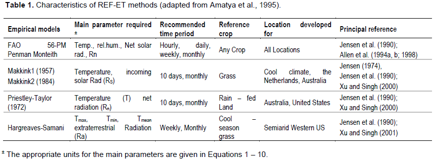
The availability of numerous equations for determination of ET, the wide range of data types needed, and the wide range of expertise needed to use the various equations correctly make it difficult to select the most appropriate evaporation method for a given study location (Xu and Singh, 2002). Therefore, the most appropriate method for a given geographical location is to be found by research on comparative studies. In the humid semi-hot equatorial climate of the lower Niger basin, comparative studies with the objective of selecting the best ETo model are lacking. The aim of this study, therefore, was to evaluate five frequently referred ETo models (Table 1) and compare them first against Epan data and secondly against FAO 56-PM (where PM stands for Penman-Monteith equation). The daily and monthly REF – ET values were calculated following examples 17 and 18, of Allen et al. (1998) on pages 70 to 73 as guide. The calculation procedures outlined in examples 17 and 18 with the sample data were first programmed in Excel spreadsheet. After the Excel calculations had accurately reproduced the results of example problems, then the example data were replaced with the study data. The study data were the routinely measured variables, maximum temperature (Tmax), minimum temperature (Tmin), mean temperature (Tmean), measured solar radiation (Rs), relative humidity (RH), wind speed (u2), and z only (where z is the elevation of the site in metres).
This study will be of great economic benefits to Nigeria, in view of the declining oil and gas revenues and the shift to agricultural economy. Most of the agricultural and allied industries are situated in remotest area without weather stations. The result of this study would be the recommendation of an empirical and less weather-data demanding REF-ET equation to FAO 56-PM which can easily be applied to such locations.
Weather station
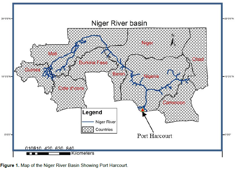
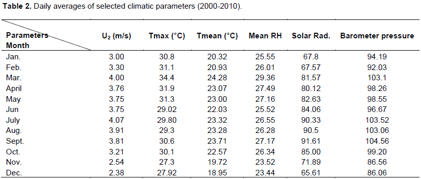
The weather station used in this study is located at the Port Harcourt International Airport, Omagwa, Rivers State, Nigeria. The station is located at latitude 04°51’N and longitude 05°35’E, elevation of 24 m (above sea level). The Nigerian Meteorological Agency (NIMET) station is equipped with the mercury and alcohol thermometers, a cup anemometer, a Campbell sunshine recorder, and a wet-bulb thermometer and some other meteorological instruments. All the instruments were checked for proper installation and operation during observations by NIMET. Figure 1 is the map of Lower Niger River Basin showing Port Harcourt while Table 2 shows the mean monthly weather characteristics for the study period. The climate of Port Harcourt may be classified as Humid Semi – Hot Equatorial Type (Salau and Lawson, 1986), with tropical wet and dry season and pronounced seasonal reversal of wind directions. The annual rainfall is greater than 3000 mm. The wet season occurs between March and October and dry season from November to February, sometimes with occasional rainfall.
Net longwave radiation ( ): The rate of longwave energy emission may be expressed quantitatively by the Stefan-Boltzman constant due to the absorption and downward radiation from the sky as:
EVALUATION OF EMPIRICAL MODEL PERFORMANCE
Quantitative methods listed in Equations 11 to 18 have been used to test the strength of and/or weakness of the different models. These methods are indicators of model performance according to Fox (1981), Willmott (1982), Douglas et al. (2009), Berengena and Gavilan (2005), Alexandris et al. (2008), Pogen et al. (2016), and Dash and Khatua (2016). These statistical measures and the regression equations were evaluated using their optimal values as benchmarks.
The results of the study are summarized in Appendix A (Tables A1 and A2), Tables 3 and 4 and Figures 2 to 7. The first stage of analysis involved the estimation of mean daily and mean monthly evapotranspiration based on Equations (1, 7, 8, 9 and 10) with their original constants. Subsequent analyses involved evaluation of REF – ET methods against FAO 56-PM and Epan data using: i) statistical measures represented by Equations (11-18), ii) statistical regression analysis, and iii) total accumulated daily and monthly ETo values and graphical plots. Tables A1 and A2 show the results of evaluation using Equations (11 to 18). In Tables A1 and A2, R represents the daily rank number for each statistical index while R* represents the corresponding monthly rank number for each statistical index. The score for each ETo method was obtained by adding the rank numbers under R or R*.
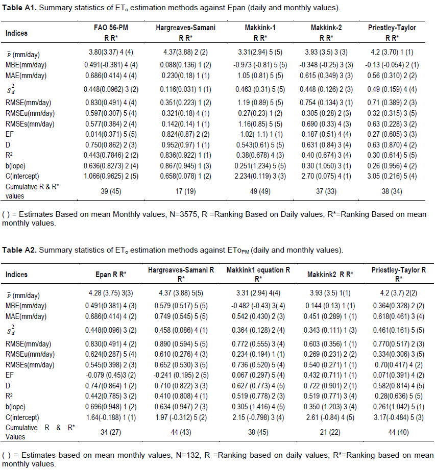
The evaluation of daily and monthly ETo estimates against Epan data are as presented in Table A1. The computed ETo values for FAO 56-PM, Hargreaves-Samani, Makkink-1, Makkink-2, and Priestley – Taylor were ranked for each of the nine indices (see column 1, Appendix A, Table A1). The cumulative ranked values of R and R* are as shown in Figure 2. Apparently, the order of ranked performance are 1st Hargreaves-Samani, 2nd Makkink-2, 3rd Priestley-Taylor, 4th FAO 56-PM and 5th Makkink-1, respectively.
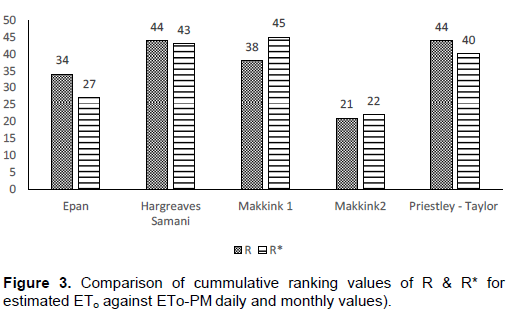
For the comparison of estimated ETo against ETo-PM for daily and monthly values (Appendix A, Table A2) The cumulative ranked values of R and R* (Figure 3) are 1st Makkink-2 with the lowest aggregate score; 2nd Epan; 3rd Makkink-1; 4th Priestley-Taylor; and 5th Hargreaves-Samani.
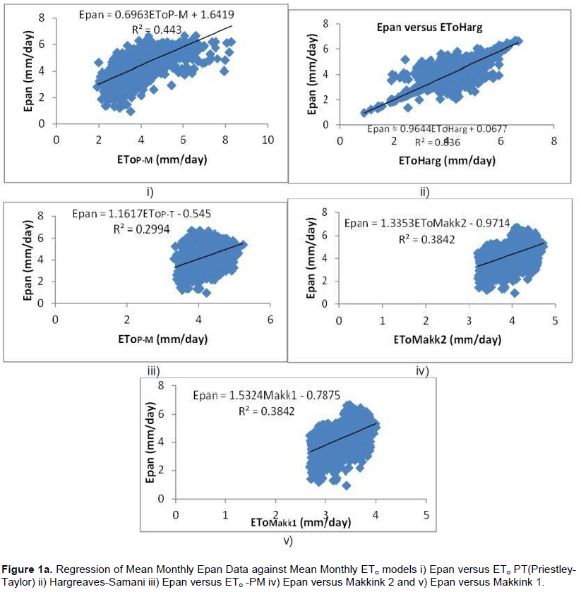
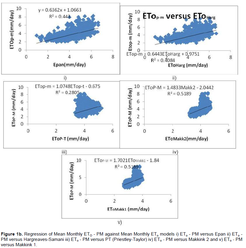
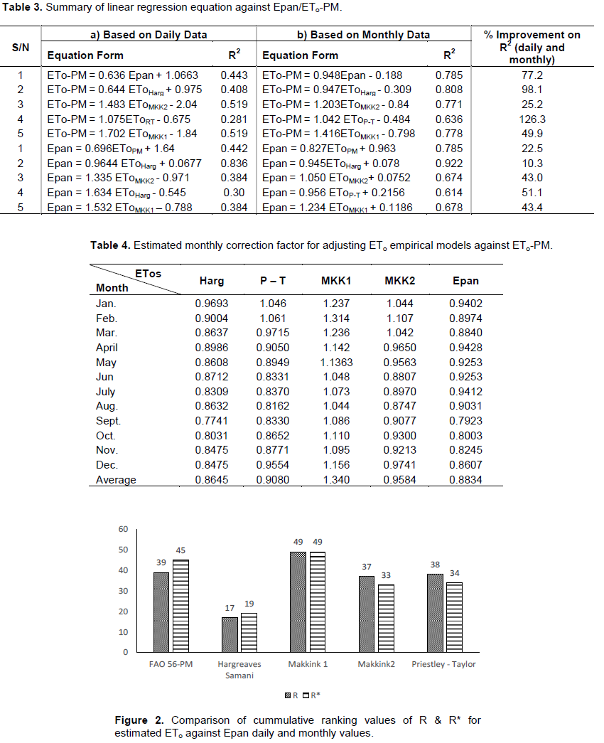
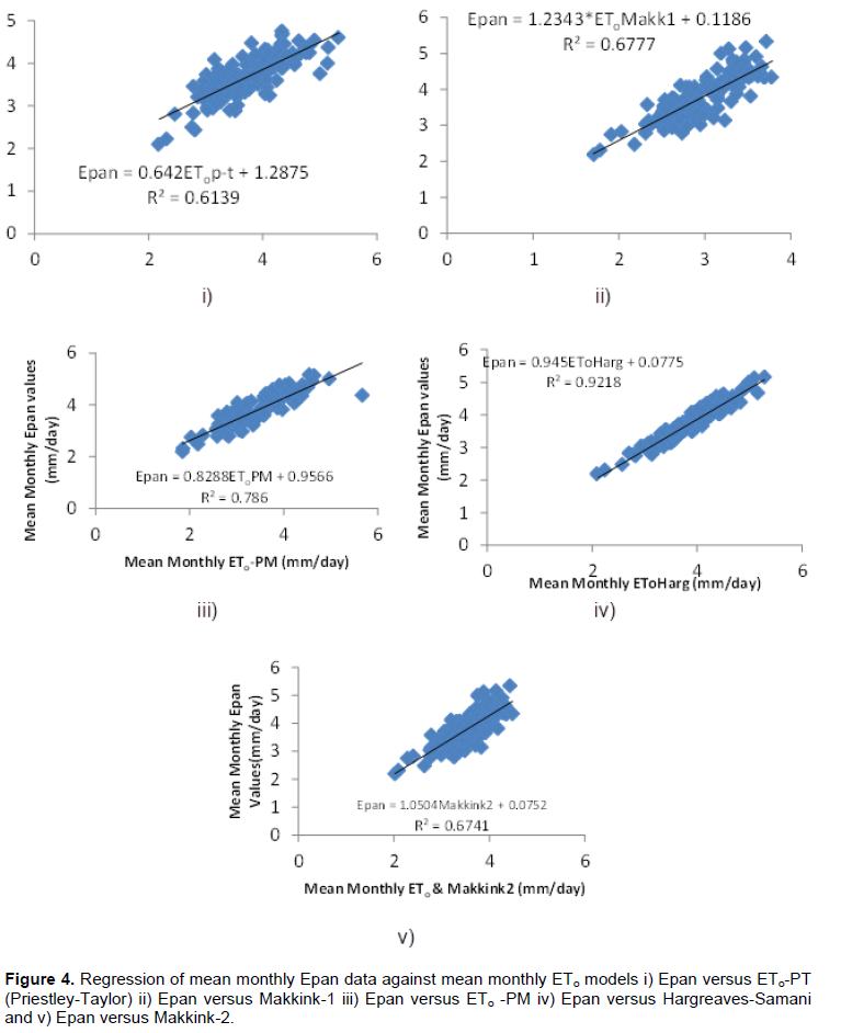
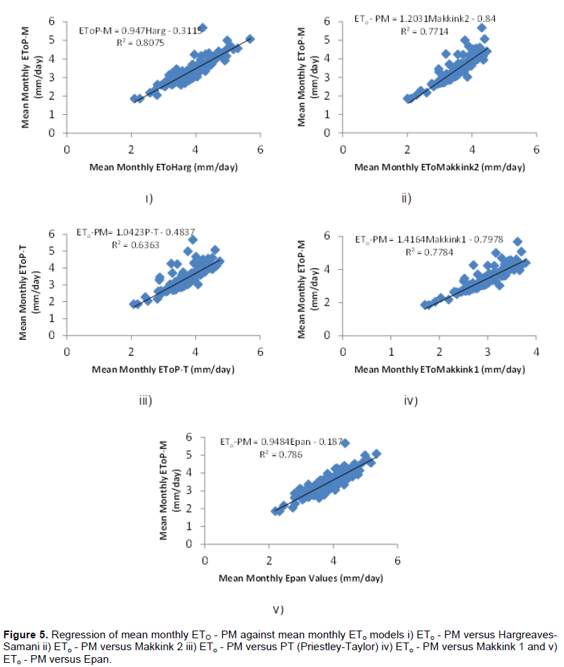
The summary of regression models of daily and monthly data are presented in Table 3. The goodness of fit of the correlation was adjudged by R2, in addition to the slope (b) and intercept (c) of the regression line. The applicable linear probability model was obtained by regressing: (i) mean daily and mean monthly, ETo-PM values against ETo values, and (ii) mean daily and monthly Epan values against ETo values. Both ETo-PM and Epan data were used as comparison criteria. A regression equation of slope (b) of 1, an intercept (c) close to zero (0) and coefficient of determination (R2) of 1, produces a perfect fit. Figures 4 and 5 show typical mean monthly plots of ETo-PM against mean monthly ETo values and mean monthly Epan values against mean monthly ETo values, respectively.
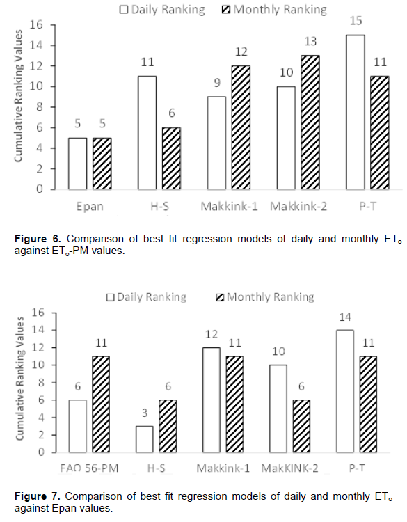
The cumulative ranked values of goodness of fit, R2, slope, b and intercept, c for the regression models (Figures 4 and 5) of daily and monthly ETo against ETo-PM or Epan values are shown in Figures 6 and 7 and Tables A1 and A2, respectively. The correlation of daily ETo values showed the following order of “best fit” (Figure 6):
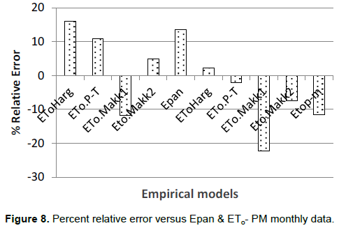
1st Epan, 2nd Makkink-1, 3rd Makkink-2, 4th Hargreaves-Samani, 5th Priestly-Taylor, respectively. For the monthly ETo against ETo-PM linear regression models, we have: 1st Epan, 2nd Hargreaves-Samani, 3rd Priestly-Taylor, 4th Makkink-1 and 5th Makkink-2, respectively. Figure 7 shows the distribution of “best fit” regression models of daily and monthly ETo against Epan values with respect of cumulative ranking of R2, b and c values. For daily ETo against Epan, the order of best fit are: 1st Hargreaves-Samani and Makkink-2, 2nd FAO 56-PM and Makkink-1, and 3rd Priestly-Taylor, respectively.
The distribution of the goodness of fit, R2 as bench mark for the various regression models are as follows: i) 0.281 - 0.519 for daily ETo versus ETo-PM; ii) 0.299 – 0.836 for daily ETo versus Epan values; iii) 0.613 – 0.922 for monthly ETo versus Epan; and iv) 0.636 – 0.808 for monthly ETo against ETo-PM values, respectively.
Figure 9 shows the cumulative monthly ETo totals for the farming season (December-April) during the study period (2000-2010). The cumulative monthly total estimated by Hargreaves-Samani was 7,136.19 mm, FAO 56-PM produced 6,448.5 mm, Priestly-Taylor- 6,538.23 mm, Makkink1- 5,298.43 mm; Makkink2- 6,280.9 mm and Epan- 7,124.32 mm.
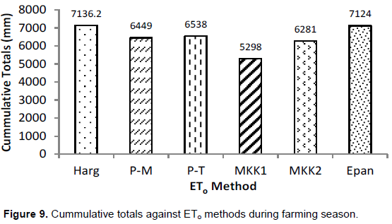
In terms of absolute values of over/under estimation and percent relative error with Epan as benchmark, Hargreaves-Samani with original coefficient over estimated by 11.87mm and percent error of 0.17% ranked first, while Priestly-Taylor; 586.1 mm and 8.23%, FAO 56-PM; 675.77 mm and 9.49%, Makkink-2; 843.38 mm and 11.84% and Makkink-1; 1825.9 mm and 25.63% ranked second, third, fourth and fifth positions, respectively. With FAO 56-PM as benchmark, Priestly-Taylor ranked best by 89.68 mm and 1.39%, Makkink-2 ranked second by 167.6 mm and 2.60%, while Epan data (675.77 mm and 10.48%), Hargreaves-Samani (687.65 mm and 10.66%), Makkink-1(1,150.1 mm and 17.84%) ranked a distant third, fourth and fifth positions, respectively.
One of the objectives of this study is to find the best and approximate alternative to the standard FAO 56-PM method. The quest for the best ETo model has prompted a global research in different climatic regions. For example, Tomar (2015) found FAO 56-PM model most appropriate for sub- humid Tarai region of Ultarakhand, India. Tabari (2010) found the Makkink model performed best in cold humid climates like the Netherlands. Amatya et al. (1995) found Turc model the best prediction method for the humid coastal plains of the United States and so on. In this study, the results of the statistical measures showed Hargreaves-Samani method ranked best for both daily and monthly evaluation with Epan data as benchmark. For the daily and monthly evaluation with FAO 56-PM as benchmark, Makkink2 (1984) ranked best while Epan data compared reasonably well with FAO 56-PM in the second position.
In terms of statistical regression analysis, Epan correlated best for daily and monthly FAO 56-PM values. Similarly, Hargreaves-Samani method correlated best with daily and monthly Epan data.
In terms of quantitative evaluation of total cumulated ETo values for the study period (2000-2010) and cumulative monthly ETo totals for the farming season (Dec-April) against both Epan data and FAO 56-PM, the results were in agreement with those of the statistical measures and regression analysis. Generally, Hargreaves-Samani method correlated best with Epan data, which is more evident in Figure 8 for the monthly ETo totals for the farming season. Hargreaves-Samani scored the overall least over estimation of 11.78 mm (11 years) and percent relative error of 0.17%. With respect to FAO56-PM, both Priestly-Taylor and Makkink-2 compared best with FAO 56-PM.
The farming season is a period of high water demand and the best performance model was Hargreaves-Samani, a plausible model for the Lower Niger basin. Similar performance of the Hargreaves-Samani has been reported by Ramirez et al. (2011) for Colombian coffee zone, although in the said study, Hargreaves-Samani was evaluated against FAO 56-PM. Also Amatya et al. (1995) found Makkink and Priestly-Taylor methods in closest agreement with FAO 56-PM. The close agreement between FAO 56-PM and the radiation-based method (Makkink and Priestly-Taylor) is probably due to the prevalent low advective conditions in the Lower Niger River basin. The study agreed with Allen et al. (1998) who recommends an alternative ETo equation to FAO Penman-Monteith equation.
The results of Equations 11 to 18 shown in Tables A1 and A2 have been used to assess the strength and weakness of the statistical measures. All the statistical measures were calculated on the basis of the relationship between observed and predicted mean deviations. The index “D” is a measure of cross-comparison between the models. Fox (1981) recommended that at least RMSE, MAE, RMSEs and RMSEu be applied in evaluating model performances and that RMSE and MAE are among the best overall measures of model performance because they summarize the mean difference between observed(O) and predicted(P) values. The criteria adopted for assessment is that values of MAE and RMSE that are very close to zero are considered better models. According to Alexandris et al. (2008), Fox (1981) and Greenwood et al. (1985) a good model is one that has very low RMSEu and RMSEs values which are close to RMSE. From Table A1, Hargreaves–Samani has the least MBE, MAE, Sd, RMSE, RMSEs values with the exception of RMSEu, thus showing the best performance against Epan, seconded by Priestly-Taylor and thirdly by Makkink2. From Table A2, Makkink2 performed best against FAO-56 PM, seconded by Epan.
The general improvement for monthly estimates in R2, MBE, MAE, and RMSE values indicated that the regression equations and statistical analyses for daily REF-ET values were less accurate than the monthly estimates. This greater error of prediction was due to the wide variation in daily weather parameters as compared to the mean monthly data where variability was reduced by the averaging effect.
In order to improve the accuracy of the REF-ET models against FAO 56-PM, monthly correlation factors have been computed as ratio of monthly total of PM REF-ET to the monthly total for each model as shown next.
Recalibration of model constants
From the evaluation of ETo models against Epan data as benchmark, only Hargreaves-Samani and Priestly-Taylor methods over estimated/under estimated with a small margin of 313.4 mm and 452.3 mm in 11 years (2000-2010). With FAO 56-PM as a bench mark, only Makkink-2 (1984) method over estimated with a small margin of 512.4 mm, the other empirical models produced large margins. The existence of large margins support the need to adjust the models in a calibration process. The adjustment was achieved with the use of mean monthly correction factors. The mean monthly correction factors for ETo models were computed as the ratio of the monthly total of FAO 56-PM to the monthly total for each method averaged over the record period (Amatya et al., 1995). Table 4 contains the estimated monthly correction factors for adjusting the ETo models against FAO 56-PM. These adjustment factors can be used for prediction of RET- ET beyond year 2010.
The following conclusions were drawn from the results of the study:
i) Based on the statistical analyses, regression analysis, accumulated REF-ET values (2000 to 2010); monthly REF-ET estimates (summed daily values) for the farming season (Dec to April). Hargreaves-Samani method was in best agreement with daily and monthly Epan data. Furthermore, Hargreaves-Samani method was in best agreement with Epan data during the farming season (December - April) producing a slight over estimation of 11.87 mm and percent relative error 0.17% in 11 years.
ii) The comparison of REF-EF estimates with Epan data and FAO 56-PM as benchmarks showed that Hargreaves-Samani method was in best agreement with Epan data while Priestley-Taylor ranked best against FAO 56 PM, seconded by Makkink2 (1984) and thirdly Hargreaves-Samani method. Thus, Hargreaves-Samani performed reasonably well with FAO56-PM.
iii) The mean monthly data correlates better with Epan data and FAO 56-PM than the daily data. The three best REF-ET models are in this order: Hargreaves–Samani, Priestley-Taylor and Makkink (1984) and may be recalibrated using the approach stated above.
iv) The FAO – 56 PM is universally accepted the “standard” method for estimating daily or monthly ETo. A major disadvantage to the application of the standardized FAO-56 PM procedure is the relatively high data demand requiring measurements of Temperature, Rel. hum., Rs, wind speed(u) and a plethora of intermediate parameters. Another problem is linked with data quality. Lastly, another serious problem is related to the cost of instrumentation for collecting the required meteorological in automated weather stations (Valiantzas, 2013; Jensen et al., 1997; Allen, 1996). The outcome of this study corroborates with Allen et al. (1998) which recommends Hargreaves-Samani as an alternative model for ETo. Hargreaves-Samani is a temperature–based model which requires only a few input parameters such as mean temperature, minimum temperature, maximum temperature and extraterrestrial radiation (Ra). Consequently, it is an economic alternative.
The authors have not declared any conflict of interests.
REFERENCES
|
Alexandris S, Stricevic R, Petkovic S (2008). Comparative analysis of reference evapotranspiration from the surface of rainfed grass in Central Serbia, calculated by six empirical methods against the Penman-Monteith formula. Euro. Water 21/22:17-28.
|
|
|
|
Allen GR (1996). Assessing Integrity of weather data for reference evapotranspiration estimation. J. Irrigation Drainage Eng. 122(2):97-106.
Crossref
|
|
|
|
|
Allen GR, Pereira SL, Raes D, Smith M (1998). Crop evapotranspiration: Guidelines for computing crop water requirement. Food and Agriculture Organisation (FAO) of the United Nations. Publication No. 56, Rome. 300 p.
|
|
|
|
|
Allen GR, Pruitt WO (1986). Rational use of the FAO Blaney – Criddle Formula. J. Irrigation Drainage Eng. 112(2):139-155.
Crossref
|
|
|
|
|
Allen RG, Smith M, Perrier A, Pereira LS (1994a). An update for the definition of reference evapotranspiration. ICID Bull. 43(2):35-92.
|
|
|
|
|
Allen RG, Smith M, Perrier A, Pereira LS (1994b). An update for the definition of reference evapotranspiration. ICID Bull. 43(2):1-34.
|
|
|
|
|
Amatya DM, Skaggs RW, Gregory JD (1995). Comparison of Methods for Estimating REF-ET. J. Irrigation Drainage Eng. 121(6):427-435
Crossref
|
|
|
|
|
Berengena J, Gavilan P (2005). Reference ET estimation in a highly advective semi-arid environment. J. Irrigation Drainage Eng. ASCE 131(2).
Crossref
|
|
|
|
|
Dash SS, Khatua KK (2016). Sinuosity Dependency on Stage Discharge in Meandering Channels, Journal of Irrigation and Drainage Engineering, ASCE, ISSN 0733 – 9437:04016030-04016030- 12.
|
|
|
|
|
Douglas EM, Jacobs JM, Sumner DM, Ray RL (2009). A comparison of models for estimating potential evapotranspiration for Florida land cover types. J. Hydrol. Jul 15; 373(3):366-376.
|
|
|
|
|
Food and Agricultural Organization of the United Nations (1990). Report on the Expert Consultation on Revision of FAO methodologies for Crop Water Requirements, Land and Water Development, Division, Rome, Italy.
|
|
|
|
|
Fox DG (1981). Judging Air Quality Model performance : A Summary of the American Meteorological Society Workshop on Dispersion Model Performance. Bull. Am. Meteorol. Soc. 62:599-609.
Crossref
|
|
|
|
|
Greenwood DJ, Neteson JJ, Drayscott A (1985). Response of Potatoes to N fertilizer: dynamic model. Plant Soil 85:185-203.
Crossref
|
|
|
|
|
Hansen S (1984). Estimating of Potential and Actual Evapotranspiration. Nordic Hydrol. 15:205-212.
|
|
|
|
|
Hargreaves GH, Samani ZA (1981). Estimating Potential Evapotranspiration. J. Irrigation Drainage Division Proc. Am. Soc. Civil Eng. ASCE 108(3):224-230.
|
|
|
|
|
Jensen ME (1974). Consumption Use of Water and Irrigation Water Requirements, Report of the Technical Committee on Irrigation Water Requirement. Irrigation and Drainage Division ASCE, New York, N.Y.
|
|
|
|
|
Jensen ME, Burman RD, Allen GR (1990). Evatranspiration and Irrigation Water Requirement ASCE Manual and Report on Engineering Practical, No.70, ASCE, New York N.Y.
|
|
|
|
|
Jensen D, Hargreaves G, Temesgen B, Allen R (1997). Computation of ETo under non-ideal conditions. J. Irrig. Drain. Eng. 123:394-400.
Crossref
|
|
|
|
|
Makkink H (1984). tentoonstellingscatalogus. Wetering Galerie Amsterdam 16p.
|
|
|
|
|
Makkink GF (1957). Testing the Penman Formula by means of Lysimeters. J. Institute Water Eng. 11:277-288.
|
|
|
|
|
Pogen FB, Ghosh KA, Kundu P (2016). Review on Different Evapotranspiration Empirical equations. Int. J. Adv. Eng. Manag. Sci. 2(3):17-24.
|
|
|
|
|
Priestley CHB, Taylor RJ (1972). On the assessment of the surface heat flux and evaporation using large-scale parameters. Mon. Weather Rev. 100:81-92.
Crossref
|
|
|
|
|
Ramirez HV, Mejia A, Marin VE, Arango R (2011). Evaluation of methods for estimating the reference evapotranspiration in Colombian Coffee. Agronomia Columbiana 29(1):107-114.
|
|
|
|
|
Salau OA, Lawson TL (1986). Dewfall Features of a Tropical Station: the Case of Onne (Port Harcourt), Nigeria. Theor. Appl. Climatol. Springer-Verlag Netherlands 37:233-240.
|
|
|
|
|
Tabari H (2010). Evaluation of Reference Crop Evapotranspiration Equations in Various Climates. Water Resour. Manag. 24:2311-2337.
Crossref
|
|
|
|
|
Tomar AS (2015). Comparative Performance of Reference Evapotranspiration Equations at Sub-Humid Tarai Region of Ultarakhand, India. Int. J. Agric. Res. 10:65-73.
Crossref
|
|
|
|
|
Valiantzas JD (2013). Simplified forms for the standardized FAO -56 Penman – Monteith reference evapotranspiration using limited weather data. J. Hydrol. Elservier 505(2013):13-23.
Crossref
|
|
|
|
|
William H, Cooke III, Grala K, Wax CL (2008). A method for Estimating Pan Evaporation for Inland and Coastal Regions of the Southeastern US. Southeastern Geographer 48:149-171.
Crossref
|
|
|
|
|
Willmott CJ (1982). Some Comments on the Evaluation of Model Performance. Bull. Am. Meteorol. Soc. 63:1039-1313.
Crossref
|
|
|
|
|
Xu C-Y, Singh VP (2000). Evaluation and generalization of radiation-based methods for calculating evaporation. Hydrol. Process. 14(2):339-349.
Crossref
|
|
|
|
|
Xu C-Y, Singh VP (2001). Evaluation and Generalization of Radiation-based Method for Calculating Evaporation. Hydrol. Process. J. 15:305-319.
Crossref
|
|
|
|
|
XU C-Y, Singh VP (2002). Cross Comparison of Empirical Equations for Calculating Potential Evapotranspiration with Data from Switzerland. Water Resour. Manag. Kluwer Academic Publishers Netherland 16:197-219.
|
|
APPENDIX