Full Length Research Paper
ABSTRACT
This study extended the agricultural household model to explain food storage, consumption and sales behaviors of farming households in northern Uganda using two major staple grains: finger millet and beans. Using secondary data collected by the Uganda Bureau of Statistics from 782 millet and beans producing households (388 households below poverty level and 394 households above poverty level), seemingly unrelated regressions were performed and risk neutrality tests were carried out. It was found that all finger millet and beans producing households in northern Uganda were risk neutral regarding storage and sales decisions with only millet producing households below poverty line being risk averse in their consumption decisions. However, households above poverty line produced and stored more millet and beans implying that they were more food secure than households below poverty level. Therefore, strategies to boost incomes, production and prudent management of millet and beans stocks at the household level are critical for food security alleviation in northern Uganda.
Key words: Food security, household, precautionary storage, consumption, sales, price risk, Uganda.
INTRODUCTION
Numerous studies have shown that precautionary food storage behavior of households differs by income level (Jalan and Ravallion, 2001; Deininger et al., 2007; Carter and Lybbert, 2012; Michler and Balagtas, 2013). Market supply, on the other hand, depends on the volume of grain harvest which is concentrated within a few months of the year in any area, and can fluctuate widely from one year to the next depending on climatic conditions (Park, 2006). According to Ravallion (1987) and Renkow (1990), households engaged in subsistence farming do not often store food for the market, but they store for future consumption. Even when prices are anticipated to rise with a high level of certainty, such households still fail to store food to get arbitrage profits. Deininger et al. (2007) argued that the concern for food security motivates household storage even when arbitrage is unlikely to insure food consumption as opposed for consumption of “all other goods”. Meanwhile, better access to credit, for example, increases household food storage for arbitrage and decreases storage for food security purpose implying an overall positive or negative net effect on storage (Park, 2006; Michler and Balagtas, 2013).
Several explanations have been made to understand why many farming households from developing countries store a portion of their output at harvest or invest in storage (Walker and Ryan, 1990; Fafchamps, 1992). Although, storage is used in developed countries to transfer income in the period between two harvests, this is not a realized outcome for most farming households. A study by Stephens and Barrett (2011) found a positive effect of credit access by households on storage (mostly for arbitrage purposes). However, Lee and Sawada (2010) ascertained that increasing access to credit reduced household’s reliance on storage. The disparity in the above study results might be because Lee and Sawada’s study was based on the premise that grain storage was a form of unproductive savings that households undertook due to credit constraints. Arguments on inadequacy of rural capital markets seem unsatisfactory as households could still transfer income to the planting season in the form of sales cash stored-away, so long as there are functional commodity markets. The scope for the more plausible reason of inter-temporal price arbitrage is limited to farming households with marketable surplus (mostly commercial and not subsistence farmers), and absence of marked seasonal fluctuations in crop commodity prices in some developing countries (Walker and Ryan, 1990).
The importance of food security considerations in explaining household storage inventories in developing countries has been emphasized by a number of researchers. Ravallion (1987) noted that “positive stocks are observed even when expected future price falls short of spot price plus marginal storage cost”. The report adds that “…stockholders are also likely to have viewed their stocks as a desirable precaution…” Renkow (1990) expounds on this “food security” reason by attempting to model on-farm storage decisions under price risk. Results showed that even if there is no scope for price arbitrage (ΔPt = 0), positive stocks may be held due to the “food security” motive (Renkow, 1990). Only in the case of large farming households is there evidence of significant arbitrage motives for holding food stocks (Ibis).
In view of these shortfalls, Saha and Stroud (1994) developed an agricultural household model of consumption, storage, savings and labour decisions expanding the reasons for crop storage under price risk beyond speculative behaviour alone, as the commodity arbitrage proponents. Particularly, for small farming households, food storage is usually motivated by their aversion to risk and food security considerations. Despite new insights into the economics of storage, this study used crop production levels to categorize sorghum farmers. Since income plays a critical role in household food security and risk-bearing in many developing countries, it perhaps would have been more meaningful to categorize the farming households using income rather than crop production levels.
In Uganda, most households usually sell off their grain surpluses immediately after harvest, rather than during the off-season when prices are high due to lack of money and proper storage facilities (APS, 1994; Owach, 1998; FAO, 2000). This household behaviour arguably could be the cause for incessant food insecurity and poverty in rural areas among other factors. Of all regions, northern Uganda is the worst hit with chronic poverty levels reaching 26% as compared to the national average of 18% (UBOS, 2015).
Therefore, the motivation of this study was to extend Saha and Stroud’s agricultural household model to explain food storage behavior of farming households in northern Uganda using two major staple grains: millet and beans. In this study, households were categorized into two based on income: households above poverty line and households below poverty line. It was anticipated that findings from this study would have policy implications on alleviation of household food and income security in northern Uganda.
ANALYTICAL FRAMEWORK
When households anticipate that price increases will be sufficient to cover real costs of storage, they tend to store food. In this case, the typical condition for strictly positive optimal storage would be:
ψEt [p~t+1] > pt + c (1)
Where: ψ = intertemporal discount rate; Et = expectations; subscript (t) = current period; pt = current price; p~t+1 = next period price; c = unit storage cost. In Equation 1, a positive storage level will occur only if the expected discounted future price ψEt [p~t+1] is greater than the spot price (pt) plus unit storage cost (c). In Equation 1, commodity storage greater than zero will occur only if the expected discounted future price ψEt [p~t+1] is greater than the current price (pt) plus the unit cost of storage (c).
Within agricultural economic cycles, it is common knowledge that optimal choices in agricultural household models are not “separable” in situations of price risk (Sadoulet and de Janvry, 1995; Singh et al., 1986). For the case of subsistence farmers, their optimal choices are not separable because they are both consumers and producers of their own produce. In this study, the model developed by Saha and Stroud (1994) where farm household maximizes a time-wise additively separable and time-invariant utility function over a time horizon of T periods is followed thus:
Max U(.) = ΣψtU(Ct, Ot, Rt) (2)
Where: U = utility; Ct = food consumption; Ot = consumption of “all other goods”; Rt = consumption of leisure. Household’s optimal choices are made in situations of production and price risk. Thus at period (t), the price at (t+1), given by (p~t+1) is not known to the farmer.
Following Saha and Stroud (1994), it is assumed the stochastic process (p~) is a stationary Markov process, thus the probability distribution of (p~t+1) is conditional only on (pt) and not the whole history of the process. Considering these assumptions, the household’s optimisation problem is
Maxzt H = U[C, pt Mt+∆bt....+At(Lt)-c(St) lt (Lt )] +ψEt[Vt+1 (p~t+1, y~t+1 )] (3)
Where: H = optimal household choices (storage, consumption, sales, labour); C=optimal consumption choice; pt = current period price; Mt = current period sales; bt = household savings; At = household’s net labour income [≡ off-farm labour earnings minus farm labour (hired and family) expenses]; lt = Leisure; Lt = optimal labour choice [Lt ≡ (hired and family farm labour]; c=inventory cost; St = current period optimal storage; zt ≡ [Ct, Lt bt+1, St] denotes the vector of decision variables to be optimally chosen by the household; E= expectation operator at period (t). Vt+1=∑Ti=t+1ψi U[C*i,, y*i,,li(Lt)] denotes the value function, where (*) superscripts indicate optimal choices; y = Household income. Since p~t+1 is unknown to the household at period (t), the value of the function is stochastic, denoted by Vt+1[p~t+1, y~t+1].
Saha and Stroud (1994) showed the first order conditions of Equation 3, with optimal choice vector, zt* = [Ct*, Lt*, bt+1*, St*] to be:
Hct ≡ Uct - pt Uyt ≡ 0 (4a)
HLt ≡ [pt QtLt (Lt )+AtLt (Lt )+)]Uyt + lyt (Lt )Ut ≡ 0 (4b)
Hbt+1 ≡ -Uyt + (1+r) ψEt[Vyt+1] ≡ 0 (4c)
HSt ≡ -[pt + C’(St)] Uyt+ ψEt[Vyt+1 p~t+1] ≡ 0 (4d)
Where all alphabetic subscripts, except the subscript t, denote partial derivatives and 0 is the null vector of the appropriate dimension.
Estimation of the model
Following Saha and Stroud (1994), the econometric model used to explore the influence of income and other factors on quantities of millet and beans stored, consumed and sold by households in northern Uganda took the form of a system of three simultaneous equations on storage, consumption and sales. The assumption that household’s optimal choices are made in an environment of output price uncertainty implies that at period (t), price at t+1, represented by p~t+1, is not known to the household. It is assumed that the stochastic process, p~ follows a stationary Markov process, hence the probability distribution of p~t+1 is conditional on only pt, and not on the whole history of the process (Saha and Stroud, 1994). Optimal (Pareto optimality) household choices are therefore defined by:
Vt (Φ) ≡ [Ct (Φ), S t(Φ), Mt(Φ)] (5)
Where: Vt = optimal household choices; Φ = parameter vector of optimal choice; Ct (Φ), = optimal consumption choice; S t(Φ) = optimal storage choice; Mt(Φ) = optimal sales choice.
Equation 5 gives the dependent variables of the complete system. Equation 6 gives the dynamic relationship of dependent and independent variables. It was assumed that household optimal savings (bt+1), are subsumed in income in each period. From first-order conditions, optimal choices are functions of current crop price, moments of the distribution of random expected future price, price of substitutes and complements, income, education and gender of household head, location and poverty status of household as shown in Equation (6) below:
π ≡ [pt, E(p~t+1), var(p~t+1), Yt, P*, P**, Sexhh, Dist, Educ, PovL, Extn, Seas] (6)
Where, π = optimal household choice (storage, consumption and sales); E(p~t+1) = expected future price (measured by the structure E(p~t+1) = θpt); var(p~t+1) = variance of future price (as proxy for price volatility); Yt = current household income (Ushs); P* = vector of prices of substitutes of millet or beans; P** = vector of prices of complements of millet or beans; Sexhh = sex of household head (male =1; female = 0); Dist = district where household is located (1=Apac; 0=Arua); Educ = number of years spent in school for formal education (years); PovL = poverty line (1=households above poverty line; 0= households below poverty line); Extn = access to extension services (1=household visited by extension personnel; 0 = household not visited by extension personnel); and Seas = production season (1= first season 2009; 0 = second season 2008).
From Equation 5, the set up to estimate a system of seemingly unrelated regression equations would take the form:
y = βx + µ (7)
Where: y is a vector of the dependent variables (C, S, M), X is a matrix of regressors corresponding to those in Equation 5, β is a vector of parameters to be estimated, and µ is a vector of error terms. Following Saha and Stroud (1994), the structures E(p~t+1) = θpt; and var(p~t+1) = θ[pt – E(p~t)]2 = θ[pt – θpt-1]2 are then imposed on the moments of the distribution of random price, and these forms are then substituted into Equation 9. The parameter (θ) was jointly estimated from the data for households above and below poverty line. The estimation equation for storage takes the form:
St = δ1+ δ2pt + δ3θpt + δ4θ[pt–θpt-1]2 + δ5Yt + δ6PovL + δ7Pcas + δ8Pbean + δ9Dist + δ10Sexhh + δ11Educ + δ12Pfcas + δ13Extn + δ14Seas +e1 (8)
and this simplifies to:
St = bo + b1pt + b2p2t + b3p2t-1+ b4ptpt-1 + b5Yt + b6PovL+ b7Pcas+ b8Pbean+ b9Dist + b10Sexhh + b11Educ + b12Pfcas + b13Extn + b14Seas +e1 (9)
Where:
(9a) bo = δ1
(9b) b1 = δ2+ δ3θ
(9c) b2 = δ4θ
(9d) b3 = δ4θ3
(9e) b4 = -2δ4θ2
and, St = current period optimal storage (in kg); bo to b14 = estimation coefficients for the respective variables; pt = current period millet price (in Ushs per kg); p2t = current price squared (in Ushs); p2t-1= lagged price squared (in Ushs); ptpt-1 = current price times lagged price (in Ushs); Pcas = current period cassava price (in Ushs per kg); Pfcas = current period fresh cassava price (in shs per kg); Pbean = current period beans price (in shs per kg; e1 = error term. Other variables are as defined in equation (6).
The structure of the optimal consumption equation was
Ct = ao + a1pt + a2p2t + a3p2t-1 + a4ptpt-1 + a5Yt + a6PovL + a7Pcas + a8Pbean + a9Dist + a10Sexhh + a11Educ + a12Pfcas + a13Extn + a14Seas + e2 (10)
Where Ct= optimal consumption of crop in current period (in kgs); ao to a15 = estimation coefficients for the respective variables; e2 = error term. Other variables in the consumption equation are as defined in Equation 9 above. The optimal sales equation is given by
Mt = go + g1pt + g2p2t + g3p2t-1 + g4ptpt-1 + g5Yt + g6PovL + g7Pcas + g8Pbean + g9Dist + g10Sexhh + g11Educ + g12Pfcas + g13Extn + g14Seas + e3 (11)
Where Mt = current period sales (in kg); go to g15 = estimation coefficients for the respective variables; e3 = error term. Other variables in the sales equation are as defined in Equation 9 above.
Under risk neutrality, household optimal choices of millet or beans storage, consumption and sales would be unaffected by changes in the second moments of random its price. Thus, the coefficients of the quadratic price regressors, p2t , p2t-1 and ptpt-1 are tested under the joint null hypothesis for risk neutrality given by,
Ho: b2 = b3 = b4 = 0 (12)
Where: b2, b3 and b4 are coefficients of the quadratic price regressors (b2 = δ4θ; b3 = δ4θ3 and
b4 = -2δ4θ2).
DATA
This study used secondary data collected by Uganda Bureau of Statistics (UBOS) during 2008/2009 agricultural census. UBOS used a stratified two-stage sample design for small and medium-scale households. The first-stage involved selection of enumeration areas (EAs) with probability proportional to size (PPS). The second stage involved selection of households (ultimate sampling units) using systematic sampling, after stratification based on acres of cropland (UBOS 2010). The total UBOS sample size for the two study districts, Arua and Apac, was 1,090 households. Using the UBOS (2010) national poverty line equivalent to Ushs 62,545 (approx. US$34) per month per adult equivalent (in 2005/06 prices), these households were categorized into two: households below and above poverty level. After data was cleaned, only 782 households (388 households below poverty level and 394 households above poverty level) were usable in this study.
The following household data were obtained from UBOS for two crop production seasons (second season 2008 and first season 2009): quantities of finger millet and beans produced, stored, consumed and sold by households, household’s income; current and lagged crop prices of finger millet and beans; prices of substitutes and complements; level of education, age and gender of household head; household access to credit, extension services, and membership to farmers’ group/association. In addition, household size was computed based on consumption conversion factors of adult-equivalent recommended by World Health Organization (WHO) guidelines (Appleton 2001).
During data analysis, a seemingly unrelated regression (SUR) regression technique was performed to determine factors influencing quantities of millet and beans stored, consumed & sold by households to allow for non separability of household decisions. Then, household response to price risk was tested using coefficients of quadratic price regressors or post-estimation risk neutrality test.
RESULTS
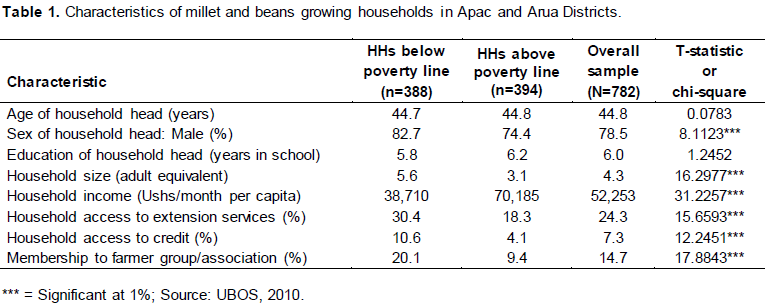
Characteristics of households
Almost three-quarters of sampled households were male headed and, there was no significant difference in age and education level of household head (Table 1). Household access to extension services, credit and membership to farmer groups or associations were generally low in the study districts, although households below poverty line appeared to have had more access to these services than their counterparts. However, as expected, households above the poverty line had higher income (Ushs 70,185 per capita per month) than those below the poverty line (Ushs 38,710 per capita per month) and, this was significant at 1% (Table 1).
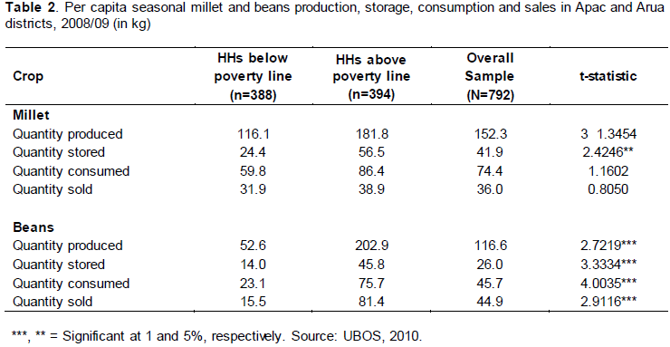
Household production, storage, consumption, and sales of millet and beans
Results in Table 2 show that households above poverty line stored significantly larger quantities of millet than households below the poverty line. The respective per capita per season storage of millet was 56.5 kg (24.4 kg) for households above poverty line (households below poverty line). There was no significant difference in per capita per season millet production, consumption and sales among household groups. For beans, households above the poverty line significantly produced, stored, consumed and sold significantly more beans than those below poverty line. Per capita per season millet production and sales for households above poverty line were 202.9 and 81.4 kg as compared to only 52.6 and 15.5 kg in the case of households below the poverty line. This indicates a better food security situation in households above poverty line than those households below poverty line.
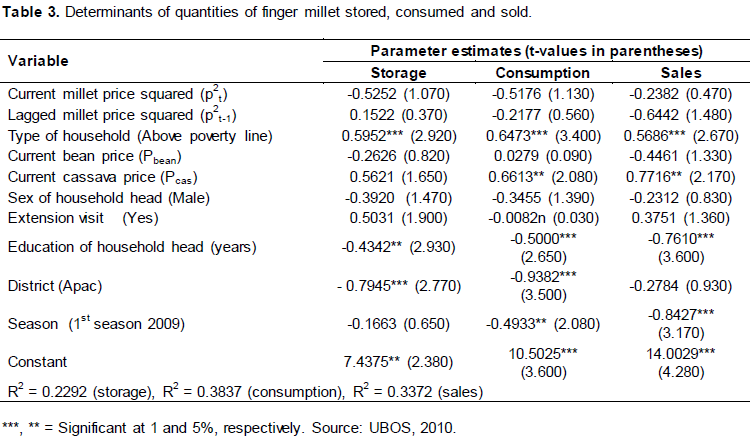
Determinants of household millet storage, consumption and sale
Results in Table 3 indicate that quantities of finger millet stored, consumed and sold varied by type of household and the result was significant at 1% level in each case. Households above the poverty line significantly stored, consumed and sold more finger millet than those below the poverty line by: storage (60%), consumption (65%) and sales (57%). Education of household head was negatively associated with quantities of finger millet stored, consumed and sold. Quantities of millet consumed and sold were positively related to the price of cassava showing that millet and cassava were complementary foods. While households in Apac stored and consumed less millet than those in Arua, household millet consumption and sales in the first season of 2009 were generally lower than in the second season of 2008. As shown in Table 3, the second moments of random price of millet (p2t and p2t-1), price of beans, sex of household head, and access to extension services did not have a significant effect on quantities of finger millet stored, consumed and sold by households.
The hypothesis that under risk neutrality, household optimal choices of storage, consumption and sales would be unaffected by changes in the second moments of random millet price was tested as in Equation 12 above and results are shown in Table 4.
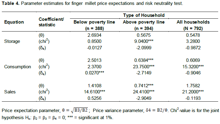
As shown in Table 4, it can be noted that finger millet growing households above poverty line were risk neutral in their storage, consumption and sales decisions. The null hypothesis of risk neutrality for storage, consumption and sales could not also be rejected for both types of households. However, households below the poverty line were risk averse in their consumption decisions.
Determinants of beans storage, consumption and sale
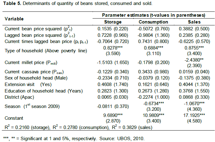
As in the case of millet, households above the poverty line significantly stored, consumed and sold more beans than those below the poverty line by: storage (83%), consumption (69%) and sales (88%). Quantity of beans sold was negatively related to the price of cassava showing that millet and cassava were complementary enterprises. Also, similar to the millet case, household beans consumption and sales in the first season of 2009 were significantly lower than in the second season of 2008. However, the second moments of random price of beans (p2t and p2t-1), product of current and lagged bean price (pt pt-1), sex of household head, access to extension services, location of household did not significantly affect quantities of beans stored, consumed and sold (Table 5).
Just like it was done for finger millet, the coefficients of the quadratic price regressors, p2t , p2t-1 and ptpt-1 under the joint null hypothesis in Equation 12 above was tested for risk neutrality of bean producing households. Results showed that the null hypothesis of risk neutrality could not be rejected for both types of households in the beans storage and sales decisions (Table 6).
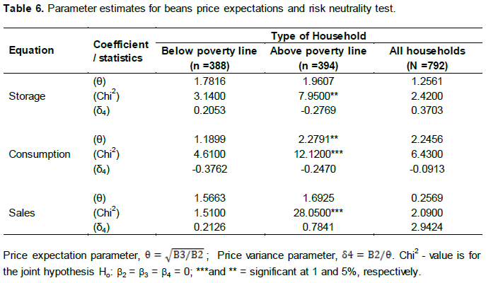
The null hypothesis of risk neutrality for beans storage, consumption and sales could not be rejected for both types of households. Thus, all beans producing households irrespective of type were risk neutral when making storage, consumption and sales decisions.
DISCUSSION
Finger millet and beans are important staple foods in northern Uganda and, their production is mainly done for subsistence purposes with only unplanned surpluses sold. These crops are grown on a seasonal basis and depending on abiotic and biotic factors, yields fluctuate by season and location. This might explain why production of millet and beans was lower in the first season of 2009 than in the second season of 2008 and, any observed disparities between study districts. Differential household resource endowments and allocation to other competing crops, such as cassava, sorghum, pigeon peas, cow peas, could have also caused variation in production, storage, consumption, and sales of millet and beans.
While this is so, previous studies have revealed that the uncertainty of future food prices and food security concerns causes more food storage as an insurance against high future price if the household has to buy back food for domestic consumption in the future (Michler and Balagtas 2013; Saha and Stroud 1994). Moreover, precautionary food storage has been found to vary with income level of households (Jalan and Ravallion, 2001; Deininger et al., 2007; Carter and Lybbert, 2012; Michler and Balagtas, 2013). Saha and Stroud (1994) found a positive relationship between household income and storage of sorghum in India. Similarly, a study of rice farmers in Bangladesh showed that higher income households stored a large portion (up to 20%) of total rice storage for precautionary purposes (Michler and Balagtas, 2013).
In northern Uganda, precautionary food storage was also significantly higher among finger millet and beans producing households above poverty level than their counterparts. Although, all finger millet and beans producing households in northern Uganda were risk neutral in their storage and sales decisions, households above poverty level seemed to be more food secure than households below poverty level. With the fact that they had more income probably enabled them to produce more millet and beans and, acquire better storage facilities for these grains.
CONCLUSION AND POLICY IMPLICATIONS
Results from this study indicate that all finger millet and beans producing households in northern Uganda are risk neutral regarding storage and sales decisions with only millet producing households below poverty line being risk averse in their consumption decisions. However, households above poverty line produced and stored more millet and beans implying that they were more food secure than households below poverty level. Therefore, strategies to boost incomes, production and prudent management of millet and beans stocks at the household level are critical for food security alleviation in northern Uganda. The establishment of minimum levels of millet and beans stocks at the household level would be a more efficient and effective policy response to any price shocks than an outright ban of household sales of these staples. For successful implementation of this policy, it will require massive promotion of use of improved storage facilities among millet and beans producing households. Using the farmer groups/associations approach, households could be mobilized and sensitized on modern millet and beans storage technologies. Moreover, household use of these improved storage technologies could be enhanced by linking them to credit and better produce markets.
CONFLICT OF INTERESTS
The authors have not declared any conflict of interests.
REFERENCES
|
APS (Agricultural Policy Secretariat) (1994). Ministry of Finance, Planning & Economic Development. Economics of Crop and Livestock Production. Kampala, Uganda: MFPED. |
|
|
Appleton S (2001). Changes in poverty and inequality in Uganda. In Reinikka R & Collier P (eds.), Uganda's recovery: The role of farms, firms and Government. Washington DC: World Bank. |
|
|
Carter MR, Lybbert TJ (2012). Consumption versus asset smoothing: Testing the implications of poverty trap theory in Burkina Faso. J. Dev. Econ. 99(2):255-64. |
|
|
Deininger K, Jin S, Yu X (2007). Risk coping and starvation in rural China. J. Appl. Econ. 39(11):1341-1352. |
|
|
Fafchamps M (1992). Cash crop production, food price volatility, and rural market integration in the third world. Am. J. Agric. Econ. 74(1):90-99. |
|
|
Food and Agriculture Organization (FAO) (2000). Increasing stockholding capabilities of smallholder farmers in Uganda. Kampala, Uganda: FAO. |
|
|
Jalan J, Ravallion M (2001). Behavioral responses to risk in rural China. J. Dev. Econ. 66(1):23-49. |
|
|
Lee JJ, Sawada Y (2010). Precautionary saving under liquidity constraints: Evidence from rural Pakistan. J. Dev. Econ. 91(1):77-86. |
|
|
Michler JD, Balagtas JV (2013). The determinants of rice storage: Evidence from rice farmers in Bangladesh. Paper prepared for the Agricultural & Applied Economics Association's 2013 AAEA & CAES Joint Annual Meeting, 4-6 August, Washington DC. |
|
|
Owach C (1998). Final report on assessment of agricultural marketing dynamics in Kitgum district. |
|
|
Park A (2006). Risk and household grain management in developing countries. Econ. J. 116(514):1088-1115. |
|
|
Ravallion M (1987). Markets and Famines. Oxford: Clarendon Press. |
|
|
Renkow M (1990). Household inventories and marketed surplus in semi subsistence agriculture. Am. J. Agric. Econ. 72(3):664-675. |
|
|
Sadoulet E, de Janvry A (1995). Quantitative development policy analysis. Baltimore: John Hopkins University Press. |
|
|
Saha A, Stroud J (1994). A household model of on-farm storage under price risk. Am. J. Agric. Econ. 76(3):522-534. |
|
|
Singh I, Squire L, Strauss J (1986). Agricultural household models. Baltimore, John Hopkins University Press. |
|
|
Stephens EC, Barrett CB (2011). Incomplete credit markets and commodity marketing behavior. J. Agric. Econ. 62(1):1-24. |
|
|
UBOS (Uganda Bureau of Statistics) (2010). Uganda census of agriculture 2008/09. Volume II Methodology Report. Ministry of Finance, Planning, and Economic Development, Kampala, Uganda. |
|
|
UBOS (Uganda Bureau of Statistics) (2015). Statistical abstract 2015. Ministry of Finance, Planning, and Economic Development, Kampala, Uganda. Uganda. OXFAM, Kampala, Uganda. |
|
|
Walker TS, Ryan JG (1990). Village and household economies in India's semi-arid tropics. Baltimore, John Hopkins University Press. |
|
Copyright © 2024 Author(s) retain the copyright of this article.
This article is published under the terms of the Creative Commons Attribution License 4.0


