ABSTRACT
The study investigated what drives farmers’ decision not to utilise their land for cultivation. The study utilised data from Statistical Office of Kosovo (SOK) with sample size of 4187 agricultural households. To achieve the objective, distance and transaction costs were examined, controlling for socioeconomic characteristics. The dichotomous dependent variable, dummy=1 if land fallow otherwise=0 was regressed over a set of explanatory variables. The model was estimated using both probit regression and linear probability model (LPM). Diagnostics test were performed after estimation. From the results, probit model passed almost all the tests. The results from both probit and LPM have low R2= 0.093. However, most of the explanatory variables showed a consistent sign and significance with useful insights into the determinants of land fallow decisions. The log likelihood ratio (LR) significance test from probit model confirmed the variables of interest are statistically jointly significant at 99% confidence level (p-value<0.001). The study revealed that distance and transaction costs along with socioeconomic factors significantly affect the decision to leave land uncultivated. It was concluded that probit model is better suited than LPM when the dependent variable is dichotomous. A combination of policy measures to reduce possibility of leaving agricultural fallowed was recommended.
Key words: Probit, linear probability models (LPM), distance and land use.
Emerging method for models analysis in which the dependent variables are either qualitative or limited in their range are really important and increasingly available and utilised as the basis of comparison to other models (Greene, 2003). One way this can be achieved is through the use of discrete choice probability models such as linear probability model (LPM) and probit regressions. Linear probability model (LPM) is ordinary Least Square OLS applied to dichotomous dependent variable – that is the observable phenomenon to be explained can take only discrete, not continuous values. However, LPM appears useful only in estimating a binary response model when approximating the partial effects of the explanatory variables is required. Probit is a nonlinear regression model specially designed for binary dependent variables. The advantages of this model lies with the ease in which it can be computed, the robustness and usually works well for values of independent variables near the mean (Wooldridge, 2010).
Lands use decisions have always been a topical issue in any development efforts. Perhaps, this is because land is the single most important natural resource that affects every aspect of a people’s live; their food, clothing, and shelter. According to World Bank (2007) an estimated 2.5 billion of the 3 billion rural inhabitants are involved in agriculture: 50% of them living in smallholder households and 27.7% of them working in smallholder households. The determinants of land use have being modelled by various studies. These studies used different approaches by varying the assumptions to model land use decision. Some of these studies make reference to Von Thunen theory on agricultural land use (Chomitz and Gray, 1996; Angelsen, 1999). Although these studies were mainly on change in land cover, they made use of location in terms of distance from the centre emphasizing that the distance affects production and marketing costs. The idea is to explore LPM and probit model technique to affirm or negate the applicability of these models. The estimates from both models are likened to the existing analysis for the purposes of exposition.
For example, Mmopelwa (1998) examined the proportion and factors causing fallowing in Botswana. The study revealed that farmers left land uncultivated either for it to regain soil fertility and/or due to biophysical, social and economic factors. Using the binomial probit model, Grisley and Mwesigwa (1995) investigated the socio economic factors that influence seasonal fallowing in Kigezi highlands. The study found that household’s size contributed an average of 26% of land under fallow and land fragmentation were highly associated with the land fallowing decision. The decision of farm household in land use is normally due to the interplay between various factors (Bergeron and Pender, 1999) these could be human capital like age, sex, and educational qualification size of household as well as household consumption needs. Although some of these studies utilised probit, the justification and the choice of a particular dichotomous dependent variable is hardly known. Again, the extent to which these studies examine critically the econometric related issues of this model remained very farfetched. Some of these issues may be post estimation test and the marginal effects in binary regression. According to Braimoh (2004) regression modelling helps to determine the relationship between variables especially when the variables of interest are statistically significant. I think this is only so when given the same set of data the result would remain same with different methodological approach. In models with dichotomous dependent variable, the coefficients of estimates have no direct interpretation. This estimate only maximizes the likelihood function, but their marginal effects thus.
It may be possible to accept or dismiss a model of economic behaviour on the basis of common sense or casual observation of phenomena. However, using relevant statistical tools to evaluate empirically the model’s prediction is essential for agricultural development. In econometrics field, good model should survive the process of empirical testing. The ability to understand and predict changes in land use pattern is essential for agricultural development (Beilock, 2005). For instance, do different transaction costs due to fragmentation of plots provide differential utility or returns to household on identical investment? Using appropriate analytical tool is essential for empirical testing and prediction of economic behaviour as well as policy implication. Comparing models with similar features will even provide basis to choose the most effective. The pertinent question is whether probit is simpler in application than LPM. Are there hiccups in utilising these techniques? What are the usefulness, similarities or otherwise of the marginal effects of these models? Interestingly too, an econometric approach to this type of study especially using dichotomous dependent variable appear to be scanty. Generally discrete choice model are often cast in the form index function model. According to Gujarati and Porter (2009), if the assumptions of probit regression analysis are not satisfied, certain problems like biasedness and very large standard errors may arise. These could result in invalid statistical inferences.
The pertinent questions are:
What are the similarities that exist between probit and LPM estimates?
What are the similarities between marginal effect in probit and LPM estimates?
How can post estimation result on probit and LPM be computed?
The broad objective of this study is to compare probit and LPM model in land use decision. The specific objectives include:
- Compare the estimates from probit and LPM model on the effect of distance on land use decisions.
- Compare the marginal effects of probit and LPM estimates on land use decisions.
- Explore post estimation result on probit and LPM parameter estimates.
THEORETICAL AND CONCEPTUAL FRAMEWORK
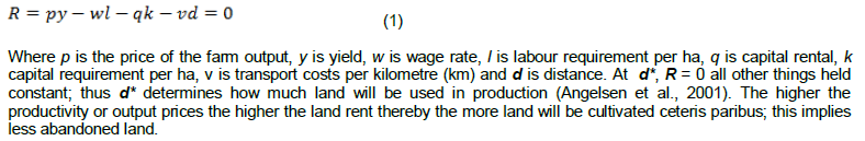
The theoretical framework utilizes Von Thunen (1960) approach combined with market imperfections utilising different assumptions as stated in Norton (1982), the land -distance theory considers land as an abundant and immobile resource and its use depends on the distance from the center (market). Following Angelsen et al. (2001), the land use depend on benefit/rent R which in addition to revenue and factor cost depends on distance as shown in Equation 1. The significance of rent (net profit) under this context is that it is the benefit to land available at a particular location above that is obtainable at the margin of cultivation which by definition is zero (Norton, 1982)

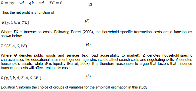
If the assumption of perfect market and abundant land is relaxed, farm household will be constrained by transaction costs, for example, due to fragmentation of land into numerous plots. Transaction may result from the cost of moving input to the farms and moving output to the markets due to scattered plots. This may be illustrated in a simple theoretical model as follows:
Hypotheses
1) Null hypothesis H0: larger distance from the farm does not influence land fallow.
2) Null hypothesis H0: farmers are not influenced by transaction costs to leave land fallow.
If we can reject the null hypotheses above at a sufficiently statistically significant level, t-values (p<0.05) then it is an indication that the variables are significant and the alternative hypothesis will be taken.
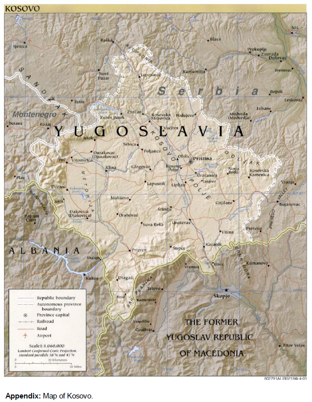
This study used primary data from a survey carried out by the Statistical Office of Kosovo (SOK) on Agricultural Household, 2005. (The choice results from the opportunity to use a complete dataset of Agricultural Household Survey). It should be noted that the time variable in this context was not important as it does not change the final result. The study examines only the applicability of this model using available data. The data contained land utilization and output data as well as agricultural households’ perceptions of barriers to land use with sample size of 4187 agricultural households. The map of Kosovo is as shown in Appendix 1. For the purpose of comparison, this study uses both LPM and the probit model. This kind of model assesses the probability of whether one or the other characteristic is present. In this instance, farmers leave land fallow=1 or y = 0 if not. Diagnostics test of specification error test was performed on the model because it was necessary to ensure that it fits the data distribution sufficiently well. Other post estimation tests namely: robustness, goodness of fit and significance test was performed after estimations. Useful transformations were carried out as well as the use of proxies.
Model specification
LPM appears useful only in estimating a binary response model when approximating the partial effects of the explanatory variables is required and cannot be relied upon to provide good estimates of partial effects for wide range covariates values (Wooldridge, 2010). Consequently, the motive of this study is not to entirely depend on using LPM but rather to use both LPM and non-linear transformation (maximum likelihood) probit.
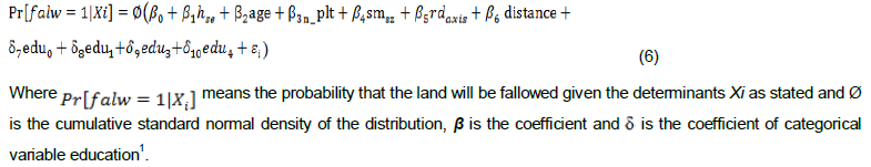
If it is assumed that land fallow Y is dependent on a number of variables as discussed and it is normally distributed with the same mean and variance, the model for estimating the land fallow is:
Goodness of fit
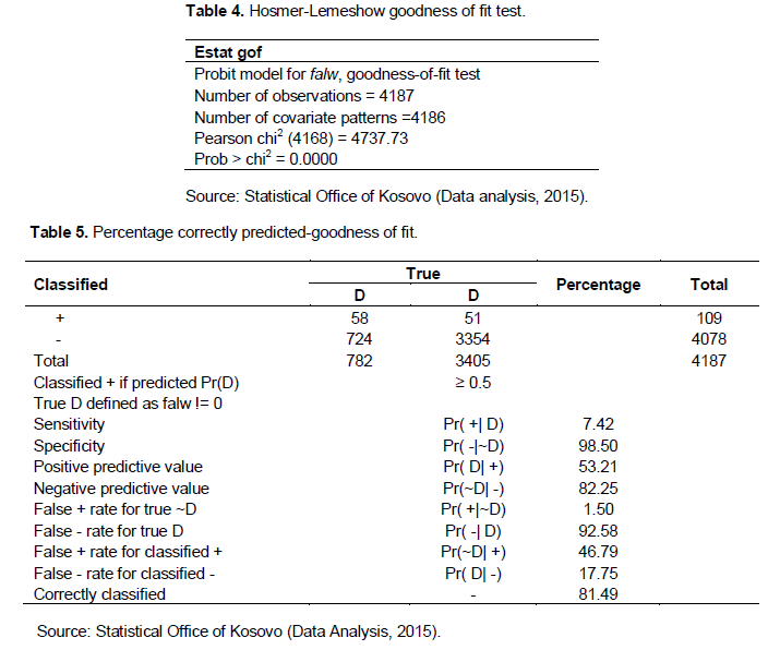
Unlike the linear regression, maximum likelihood estimation is not chosen to maximise any goodness of fit measure. Consequently, there is no reliable goodness of fit (Gujarati, 2009). However, in default, numerous measures have been proposed for comparing alternative model specification: proportion of correct prediction, sum of square residuals, pseudo R2 and Hosmer-Lemeshow or Pearson’s test Statistic. The estat classification as seen in stata output reports the proportion of correct prediction with various summary statistics as well as the classification table as shown in Table 5. It should be noted that the problem with the proportion correctly classified is that it depends on the distribution of dependent variable. Wooldridge (2010) argued that percentage correctly predicted is a useful measure for goodness of fit but was quick to point out the possibility of getting high percentage correctly predicted even when the least likely outcome is poorly predicted. The maximum likelihood ratio test is used for the joint significance of all the variables of interest, with the null hypothesis H0: all coefficients for key variables=0 analogous to the overall F-test of model significance in regression. Pseudo R-square is a bit different, it captures more or less the same thing in that it is the proportion of change in terms of likelihood.


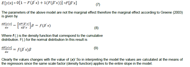
Marginal effects of Probit
Since the coefficients of probit estimation have no direct interpretation, being the values that maximize the likelihood function, according to Buam (2003), a more useful measure is the marginal effects. Given the probability model:
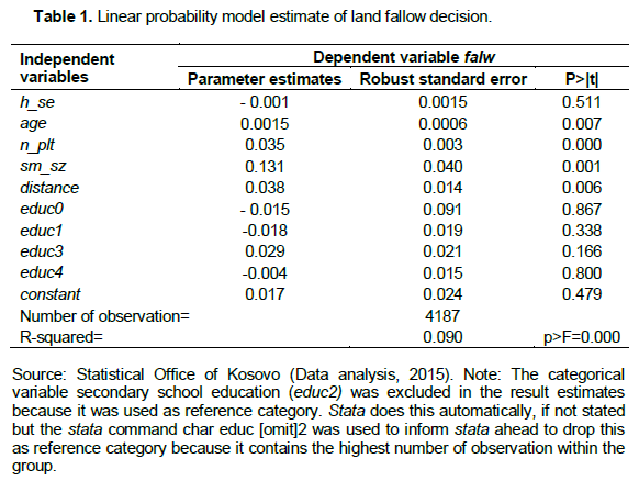
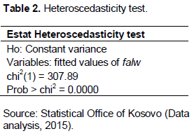
The results from LPM and probit are shown in Tables 1 and 3, respectively. The estimates from the two models are very similar. The signs of the coefficient are the same in the models with same variables being statistically significant in each model. The two models have nearly equal but not too large R2 values: 0.091 and 0.093 for LPM and probit respectively. Most of the explanatory variables showed a consistent sign and significance in the two models with useful insights into the determinants of the decision to leave land fallow. The log likelihood ratio (LR) significance test from probit model confirmed the variables of interest are statistically jointly significant at 99% confidence level (p-value<0.001). Multicollinearity is not a problem among variables because Stata does this automatically by removing perfect collinearity. The linear probability model (LPM) could not pass the diagnostics test (Table 2). This is not surprising as issues with LPM have earlier been raised. However, for the purpose of comparison this study begins with the report of the linear probability estimates.
Results from LPM estimates
From Table 1, the variables, number of plots (n_plt), distance, are individually statistically significant at 1% level while age of farm household (age), size of the smallest plot size (sm_sz), as well as the constant are both significant at 5% level. In order to interpret the estimates from LPM it must be noted that a change in an independent variable changes the probability of dependent variable, fawl=1 by a constant amount. For example, the results from the LPM revealed that, holding all other variables fixed, a rise in farm income decreases the probability of land fallow by 0.8% ceteris paribus. However, an increase in the age of household head is associated with 0.15% increase in the probability of leaving land fallow ceteris paribus. Transaction proxies, number of plots and smallest size of plot are positively related to land fallow decisions. An additional number of plot increases the probability of land fallow by 3.5%. In the same vein, size of the smallest plot size increases the probability of land fallow by 13.1%. However factor endowment variables decrease the probability of land fallow.
Interpretation of the LPM above highlights one basic difference between LPM and probit; LPM assumes constant marginal effects (e.g age educ n_plt etc) while the probit implies diminishing marginal magnitude of the partial effects. For instance, Table 3, an additional year of age is estimated to increase the probability of land left fallow by approximately 0.15%, ceteris paribus, regardless of how many plots the household was initially operating and regardless of other levels of other explanatory variables like number of plots and education. This is better imagining than real. One would expect that the probability is non-linearly related to years of experience. At a very low level of experience say fewer than 16 years, a household will not leave land fallow (cannot even own a land let alone leaving land fallow) but at working age of say 16 to 64 years, it is most likely that land will be left fallowed. Any increases in beyond 90 years, which is the maximum age of household will have little effect on the probability of land fallow. Thus, at both end of the distribution the probability of leaving land fallow will be virtually unaffected by a marginal increase in years of age.
Another related issue is that LPM violates the assumption of normal distribution of the error term and heteroscedasticity condition, meaning the variance of the disturbance is not constant. As a result, OLS is inefficient and the t and F statistics is generally invalid. Perhaps this explains why the LPM failed the hetroscedasticity test (Table 2). This suggested that LPM models might not be suitable for estimation when the dependent variable is dichotomous but may only provide an insight into a binary regression model. Hence, the detailed discussion is done under probit model. What follows next is the probit model discussion.
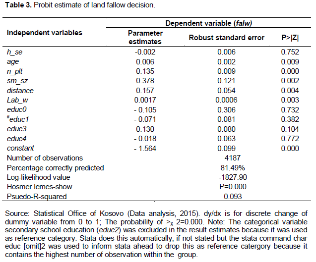
Results from probit estimates
As earlier mentioned, the coefficients of probit estimation have no direct interpretation (being simply the values that maximize the likelihood function), however the marginal effects does. The coefficients give the sign of the partial effects of each Xj on the response probability. As presented in Table 3, the coefficient for variable (n_plt) is positive. This means an increase in number of plots owned by farm household increases the probability of land fallow ceteris paribus. This is an indication that additional number of plots is associated with land fragmentation. Land fragmentation involved moving input and output between the scattered plots, incurring transaction costs in the process of negotiating, getting information thereby, reducing the incentive to utilizing more land with resultant effect of leaving land fallow as earlier mentioned. Thus, a transaction cost is crucial. Also, the second transaction costs proxy, size of smallest plot (sm_sz) is positive and highly significant. This means having smaller size of plots increase the probability of land left fallowed ceteris paribus. The significance of this variable along with the significant of number of plots owned by a farm household corroborates our argument that transaction increases fallow. If transaction costs are high farmers may not participate in market (Bergeron and Pender, 1999) thus resulting in land left fallow.
As for the dummy variable distance, the coefficient is positive and highly significant. This means that holding all other factors of fixed municipalities farther from highway are associated with increase in land fallow compared to those that are linked to highway. This is an indication that farm households farther from market are likely to leave more land fallow compared to those closer to the market (with access to market). Another related reason for this could be that farmers close to market are expected to cover less distance costs as suggested by theoretical framework (Von Thunen, 1966) cited in Norton, (1982). This could generate more rent as they cover less distance costs such that less land is fallowed. According to Norton (1982), land is abundant but its use depends on distance from the market. This appears to justify the physical role played by distance and transactions costs as discussed earlier thus, demonstrating the effect of distance and heterogeneity in productive capability.

The significance of transaction cost and distance may suggest that these factors may have increased the costs of production and marketing and decrease the incentives to use all land available thereby leaving agricultural land fallow. According to Barret (2008) when farm households are exposed to factor market imperfections and constraints, access to market involve transaction costs. This may be an indication of imperfect markets.
Post estimation tests results
The R- squared for the LPM was the usual R-squared reported for ordinary least square (OLS) (Table 1). In the case of probit model, it employs maximum likelihood estimation; therefore, there is no direct goodness of fit measure. The values for measures of fit in Table 3 from estimates showed the Psuedo R2 value 0.093. However, using another measure of fit- the Hosmer-Lemeshow goodness of fit test (HGFT)- as presented in Table 4 (p-value<0.001), the result showed that there was no significant difference between the observed and predicted number of successes and thus the model fits the data well. In Stata the command estat gof was used for this test. Additionally, the estat classification as seen in Table 5 (which is another measure of goodness of fit) is used for percentage correctly predicted. It correctly predicts ‘land fallow’ 81.49% of the time. It should however be noted that it is possible to get high percentage correctly predicted even when the least likely outcome is poorly predicted (Wooldridge, 2010), which can sometimes be misleading. The varying R2 (between pseudo R2, HGFT and percent correctly predicted) is an indication that the model used is not chosen to maximize any goodness of fit in models where the dependent variable is dichotomous. Consequently, one should not overplay the importance of goodness of fit in models where the dependent variable is dichotomous.
From the discussion so far, the positive significance of both distance and transaction costs may suggests that these factors may have increased the costs of production and marketing and decrease the incentives to use all land available thereby leaving agricultural land to fallow. This goes to show that distance in relation to other factors costs matters too. The larger the distance from market, the more land that has been allowed to fallow as rent also decreases (due to rise in transport costs) as suggested by the theory.
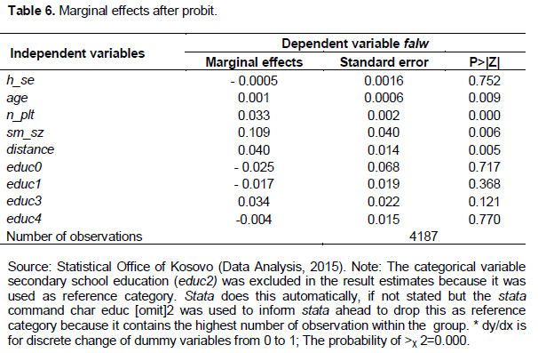
Results of marginal effects after probit
The marginal effects after probit estimates are presented in Table 6. As earlier discussed, the estimates from linear probability and probit models were not directly comparable but the marginal effects were comparable.

The results from LPM and marginal effects after probit estimates were very similar. For example, the results revealed that the marginal effect for age was 0.0010 and is significant at 5% probability level. This observation means that a marginal change in age from the average of 36.4 years in the age of household head was associated with 0.15% increase in the probability of leaving land fallow. The result of estimated coefficient was almost same with estimates from LPM in Table 1. The dummy variable distance, was associated with 4% lower land fallow ceteris paribus. An additional number of plots (n_plt) increased the probability of land fallow by approximately 3.3% ceteris paribus. In the same vein, a rise in h_se decreases the probability of land fallow by 0.6% ceteris paribus. The marginal effect after probit discussed above was obtained using mfx and dprobit command. The resulting estimates obtained from these two commands are similar, in short, same results.
While bearing these in mind, the categorical variable educational attainment (educ), generally decreased fallow at various levels but educ was not significant in both models (LPM and probit). Firstly, the marginal effect of primary school education (educ1) was -0.025. The observation means educ1 was associated with 2.5% lesser land left fallow compared to the base category2 ceteris paribus. Similarly, the marginal effect of university education (educ4) was -0.004. The observation means educ4 was associated with 0.4% lesser land left fallow compared to the base category ceteris paribus. This was an indication that additional qualification decreases the probability of leaving land fallow. However, the link between high school educations (educ3) was rather surprising. The marginal effect was 0.034 and positive. This means that educ3 was associated with 3.4% higher land left fallow. One possible reason for this could be that educated farmers have acquired knowledge in relation to improved methods of land management with the ability to acquire loans for increased farm activities through investment in land improvement practices and are also capable of diverting the resources to non-agricultural activities perceived to offer higher returns thus compounding liquidity constraints.
2The base category as mention earlier is Secondary school education (educ2)
The signs of the coefficient are the same in both models with same variables being statistically significant in each model. Since the variables included are statistically individually significant at p<005 from their respective t-values we reject the null hypothesis that these variables are not statistically significant. Based on the findings, the decision of whether land is fallowed or not is premised upon the interplay of factors, the distance and transaction costs. While the probit model passed almost all the diagnostics tests performed, the LPM did not. Thus, probit model may be better suited than LPM when the dependent variable is dichotomous. The combination of statistical significance with relatively low fit is typical for models explaining individual behaviour. Given the findings, it is recommended that probit model should be utilized when dependent variable is dichotomous and a combination of policy measures that will enhance renting of distant plots should be adopted.
The authors have not declared any conflict of interests.
REFERENCES
|
Angelsen A (1999). Agricultural expansion and deforestation: Modelling the impact of population, market forces and property rights. J. Dev. Econ. 58(1):185-218.
Crossref
|
|
|
|
Angelsen A, van Soest D, Kaimowitz D, Bulte E (2001). Technological change and deforestation: A theoretical overview, in Angelsen A, Kaimowitz D (eds) Agricultural Technologies and Tropical Deforestation. CABI Publishing Association Centre Int. For. Res. pp. 19-34.
Crossref
|
|
|
|
|
Barrett CB (2008). Smallholder market participation: Concept and evidence from eastern and southern Africa. J. Food Policy 33:299-317.
Crossref
|
|
|
|
|
Beilock R (2005). Rethinking agriculture and rural development in Kosovo, South-Eastern Europe. J. Econ. 3(2):221-248.
|
|
|
|
|
Bergeron G, Pender J (1999). Determinants of land use change: evidence from a community study in Honduras. Environment and Production Technology Division, International Food Policy Research Institute (EPTD) Washington. Discussion paper no. 46.
|
|
|
|
|
Braimoh KA (2004). Modeling Land use change in the Volta Basin of Ghana, Cuilliar Verlag, Gottingen. Ecol. Dev. Series No. 14:2014.
|
|
|
|
|
Chomitz K, Gray D (1996). Roads, land use and deforestation: A spatial model applied to Belize. World Bank Econ. Rev. 10(3):487-512.
Crossref
|
|
|
|
|
Data Analysis (2015). Available at:
View
|
|
|
|
|
Greene WH (2003). Econometric Analysis, 7th Edition, Prentice Hall.
|
|
|
|
|
Grisley W, Mwesigwa D (1995). Socio Economic Determinants of Seasonal. Fallowing. J. Environ. Manage. 42:81-89.
Crossref
|
|
|
|
|
Gujarati D, Porter D (2009). Basic Econometrics, 4th Edition, McGraw-Hill.
|
|
|
|
|
Mmopelwa G (1998). Factors contributing to land fallowing in a permanent cultivation system. J. Arid Environ. 40(2):211-216.
Crossref
|
|
|
|
|
Norton W (1982). The Relevance of Von Thunen Theory to Historical and Evolutionary Analysis of Agricultural Land use. J. Agric. Econ. XXX(1):39-47.
|
|
|
|
|
World Bank (2007). Kosovo Poverty Assessment. Report No. 39737-XK (Poverty Reduction and Economic Management Unit, Europe and Central Asia Region.
|
|
APPENDIX