ABSTRACT
The experiment was conducted in Northern Ethiopia from 2011-2013 under rain fed conditions in a total of seven environments vis. E1, E2, E3, E4, E5, E6 and E7. The objective of the study was to evaluate the adaptability and stability of sesame genotypes across environments. 13 sesame genotypes were evaluated and the experiment was laid out in a Randomized Complete Block Design with three replications. The average grain yield of the genotypes was 742.9 Kg/ha with the outstanding genotypes being G4 (926.8 kg/ha), G1 (895.1 kg/ha) and G12 (832.7 kg/ha) respectively, and low the yielding genotype was G9 (614.3 kg/ha). The combined ANOVA for grain yield showed significant effects of the genotypes, environments and genotype x environment interaction. According to the additive main effect and multiplicative interaction bi-plot (AMMI bi-plot) and Genotype x Environment interaction bi-plot (GGE bi-plot) G12 was the most stable, and G7, G8 and G9 were the unstable genotypes. Furthermore, the Genotype main effects and GGE bi-plot showed E5 as the most discriminating and representative environment. The GGE bi-plot also identified two different growing environments, the first environment containing E4 and E6 (in the Dansha area) with the wining genotype G1; and the second environment encompassing E1, E2, E3, E5 and E7 (in the Humera, Dansha and Sheraro areas) with winning genotype of G4.
Key words: AMMI bi-plot, environment, GEI, GGE bi-plot.
Sesame (Sesamum indicum L.) is an ancient oil seed crop known and used by man.It is not clearly known where Sesame originated and different scholars declare different regions as the centers of origin of this crop. However, Ethiopia is recognized as a center of diversity for this crop owing to the highly diversified sesame types present in the country.
According to FAOSTAT (2012), Ethiopia is the sixth largest sesame producer in the world and third in Africa following Myanmar, India, China, Tanzania and Uganda.
The productivity of sesame in Northern Ethiopia (specifically in the study area) is very low (525 kg/ha) compared with the national average yield of about 757 kg/ha in 2012/13production year (CSA, 2013) as well as with the world average yields, especially countries like Mozambique which produce up to 1500 kg/ha (Buss, 2007). On-top of this problem the quality of sesame seeds is deteriorating from time to time which may negatively affect the important traits of Humera sesame such as its seed color aroma and seed size uniformity. Sesame genotypes grown in Ethiopia, including the released varieties, are highly variable when grown across locations. Hence, it is important to test different newly introduced genotypes or released varieties across locations.
According to Ceccarelli (2012) the response of genotypes across environments may be with no interaction, quantitative interaction or qualitative interaction. GEI (Genotype x environment interaction) occurs when different genotypes respond differently to different environments and it is familiar in agricultural research (Allard and Bradshaw, 1964). Sesame is a short day plant and sensitive to photoperiod, temperature, moisture stress, water logging and different management practices and its yield and yield attributes are not stable and vary widely over different environments. Hence, this experiment was undertaken to identify stable and high yielding genotype(s) and to recommend best Sesame genotype(s) for the different sesame growing areas so as to boost sesame production and productivity in these (study areas) sesame belts.
In the presence of significant GEI, there are a number of univariate and multivariate stability measures used to identify stable and high yielding genotypes. Additive main effect and multiplicative interaction (AMMI) is important to analyze multi-environment trials (METs) data and it interprets the effect of the genotype (G) and environments (E) as additive effects and the GEI as a multiplicative component (which are sources of variation) and submits it to principal component analysis (Zobel et al., 1988). Another multivariate stability measure called Genotype main effects and Genotype x Environment interaction (GGE) effects is also important to identify mega-environments, the “which-won-where” pattern, and to evaluate genotypes and test environments (Yan et al., 2007).
Procedure
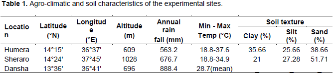
The experiments were conducted in North western and Western Tigray, Northern Ethiopia, under rain fed condition, from 2011-2013 in Humera and Dansha areas, and in 2013 cropping season in Sheraro (a total of seven environments); E1, E2, E3 are 2011, 2012, 2013 growing seasons respectively in Humera; E4, E5, E6 are 2011, 2012, 2013 growing seasons respectively in Dansha; and E7 is 2013 growing season in Sheraro. Some characteristics of the study areas are given in Table 1. Thirteen sesame genotypes (Acc#031 (G1), Oro (9-1) (G2), NN-0079-1(G3), Acc-034 (G4), Abi-Doctor (G5), Serkamo (G6), Acc-051-020sel-14 (G7), Tate (G8), Acc-051-02sel-13 (G9), Adi (G10), Hirhir (G11), Setit-1 (G12), Humera-1(G13)), brought from WARC (Werer Agricultural Research Center), were sown in RCBD with three replications. Each genotype was randomly assigned and sown in a plot area of 2.8 m by 5m with 1m between plots and 1.5 m between blocks keeping inter and intra row spacing of 40 cm and 10 cm, respectively. Each experimental plot received all management practices equally and properly as per the recommendations for the crop.

Statistical analysis
Homogeneity of residual variances was tested prior to a combined analysis over locations in each year as well as over locations and years (for the combined data) using Bartlet's test (Steel and Torrie, 1980). Accordingly, the data collected were homogenous and all data showed normal distribution.
A combined analysis of variance was performed from the mean data of all environments to detect the presence of GEI and to partition the variation due to genotype, environment and genotype x environment interaction. Moreover, mean comparison using Duncan's Multiple Range Test (DMRT) was performed to explain the significant differences among means of the genotypes. GenStat 16th edition (GenStat, 2009) statistical software was used to analyze the combined mean of the different traits of the genotypes. The model employed in the analysis was;
Yijk = μ + Gi+ Ej+ Bk + GEij+ εijk
where: Yijk is the observed mean of the ith genotype (Gi) in the jth environment (Ej), in the kth block (Bk); μ is the overall mean; Giis effect of the ith genotype; Ejis effect of the jth environment; Bk is block effect of the ith genotype in the jth environment; GEij is the interaction effects of the ith genotype and the jth environment; and εijk is the error term.
Abi-plot showing the genotype and environ mental means against Interaction Principal component analysis one (IPCA1) (AMMI1 bi-plot), and Interaction Principal component analysis one (IPCA1) against Interaction Principal component analysis two (IPCA2) (AMMI2 bi-plot) was also performed using AMMI model using GenStat software.
A GGE bi-plot was also executed using GGE bi-plot in the Meta analysis of GenStat 16th edition. This methodology uses a bi-plot to show the factors (G and GE) that are important in genotype evaluation and that are also the sources of variation in GEI analysis of MET (Multi-environment trial) data (Yan, 2001). Moreover, mean comparison using Duncan's Multiple Range Test (DMRT) was performed to explain the significant differences among means of genotypes and their traits.
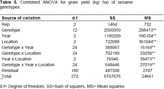
Combined Anova and estimation of variance components
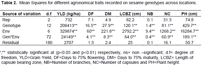
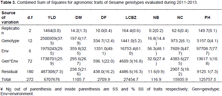
The results obtained from the combined analysis of variance of all the evaluated traits and genotypes is illustrated in Table 2. The genotype, environment and genotype x environment interaction (GEI) variance were decomposed to provide a general overview in relation to the evaluated traits and overall performance of the genotypes (Tables 2 and 3). Accordingly, the genotypes, the environments and the genotype x environment interaction components showed highly significant variation (p<0.001) for all agronomic traits. This statistical difference confirms that the difference of the traits was due to both the main and interaction effects. Zerihun et al. (2011) also found similar results of the genotype, environment and genotype x environment interaction effects in barley land races. On top of the genetic variability, the ANOVA also revealed that the environments (both locations and growing seasons) on which the experiments were conducted were different from one another in treating the genotypes. Moreover, it also indicates that the response of the genotypes were unstable and fluctuated in their trait expression with change in the environments. This phenomenon clearly confirms the existence of GEI in this study. For most of the traits the contribution of environment for the overall variance was high (ranging from 29.5% for grain yield to 77.7% for plant height) followed by genotype × environment interaction and genotype respectively.


Similar results were reported by Hagos (2009); Ahmed and Ahmed (2012). With respect to grain yield, the greatest source of variation was mainly the inherent genetic component meaning genotypic effect (37.3 %) (Table 3) which is similar to the results reported by Zenebe and Hussien (2009) and John et al. (2001)..
Agronomic performance of Sesame genotypes
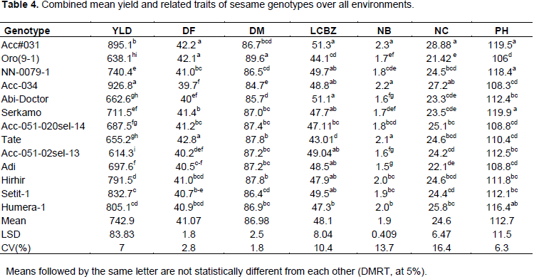
The average grain yield of the tested sesame genotypes over the seven environments was 742.9 kg/ha. G4 had the highest average grain yield (926.8 kg/ha) followed by G1 (895.1 kg/ha) while G9 was the lowest yielding genotype (614.3 kg/ha) (Table 4). G4 had early flowering (39.7 days) and early maturing (84.7 days). On the contrary, G8, G1, and G2 were late flowering genotypes (Table 4). Similarly G2 was the latest maturing genotype (89.6 days) followed by G8 and G11 which took on average of about 87.8 days each to reach maturity. The shortest (43.01cm) and longest (51.27 cm) average length of capsule bearing zone was recorded from G8 and G1 respectively. G1 also had the highest number of branches and number of capsules whereas G10 and G2 had the lowest (table 3). G1 (119.5 cm) and G6 (119.9 cm) were the genotypes with longest stature.
Variance estimate of grain yield of the genotypes
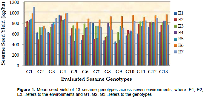
The combined ANOVA for grain yield revealed that there were highly significant variation (p<0.01) among the genotypes, environments (year, location, year x location) and genotype by environment interaction (Genotype x Year, Genotype x Location and Genotype x Year x Location) (Table 5). These significant variations of the genotypes, environments and the GEI indicated that the response of the genotypes were unstable and fluctuated in their grain yield with change in environment and these phenomenon clearly confirmed the presence of GEI in this study. Figure 1 depicts clearly the fluctuation of the genotypes across the environments. The grain yield of the thirteen genotypes was highly fluctuating over the seven environments showing highest grain yield cross-over interaction from environment to environment.

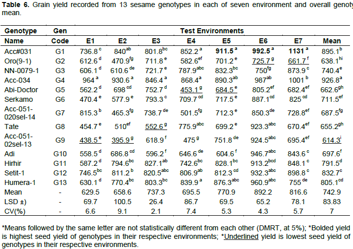
Among the environments the highest seed yield (1131 kg/ha) was observed from genotype G1in environment seven (E7) and the lowest seed yield (395.9 kg/ha) was recorded from genotype G9 in environment two (E2) (Table 6).
AMMI model
The AMMI model is fully informative for both the main effect as well as for the multiplicative effects, for clearly understanding GEI (Zobel et al., 1988). In addition to the usual ANOVA the ANOVA from the AMMI model for grain yield also detected significant variation (p<0.001) for both the main and interaction effects indicating the existence of a wide range of variation between the genotypes, years (seasons), locations and their interactions.
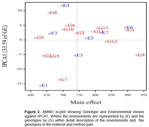
AMMI1 bi-plot analysis
The AMMI bi-plot analysis provides a graphical representation to summarize information on main effect and interaction effects of both genotypes and environments at the same time.The AMMI1 bi-plot containing the genotype and environment means against interaction principal component analysis one (IPCA1) scores is illustrated in Figure 2. As indicated in Figure 1 the displacement along the abscissa reflected differences in main effects, whereas displacement along the ordinate exhibited differences in interaction effects. Genotypes and environments with IPCA1 greater than zero are classified as high yielding genotypes and favorable environments whereas those with IPCA1 lower than zero are classified as low yielding genotypes and unfavorable environments (Yan and Thinker, 2006). Accordingly genotypes such as, G1, G4, G11, G12 and G13 were the genotypes with above average mean grain yield as they laid-down on the right side of the vertical line (grand mean of the genotypes and environments). Conversely, genotypes G2, G5, G6, G7, G8, G9 and G10 had below grand mean because they laid down to the left side of the vertical line. Exceptionally, G3 laid down very close to the vertical line, indicating the mean yield of G3 was highly similar over all environments and parallel to the grand mean of all genotypes. G4 followed by G1 had higher mean yield in the favorable environments, whereas G9 and G2 had lower mean yield in the unfavorable environments. Regardless of their contribution for the interaction, G8 and G5 fall on the same vertical line (ideal) showing their similarity in their mean yield. G1 and G10 which laid down on the same horizontal line had similar contribution in the interaction component despite of their yield performance.

Regarding the environments, E5, E6 and E7 had above the grand mean grain yield and were considered as favorable environments. On the other hand, E1, E2 and E4 had below average grain yield and were considered as unfavorable environments. E3 laid down very close to the grand mean line indicating that genotypic yield in E3 represents the overall genotypic mean across all environments.
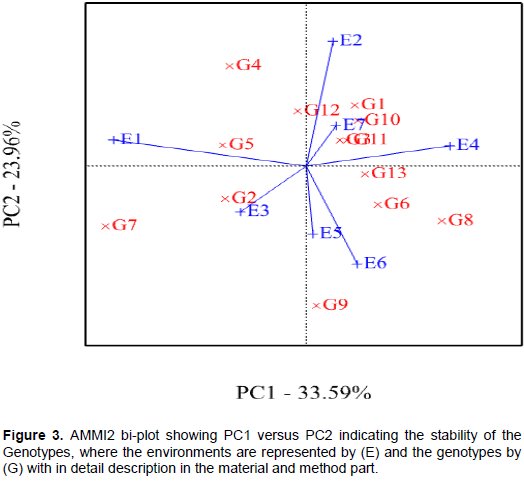
AMMI 2 bi-plot: The AMMI 2 bi-plot, containing IPCA1 in the X-axis and IPCA2 in the Y-axis, is plotted in Figure 3. The first interaction principal component (IPC1 or PC1) contained 33.59% and the second interaction principal component (IPC2 or PC2) explained about 23.96% and the two interaction principal components cumulatively explained about 57.55% of the sum of squares of the genotype by environment interaction of the genotypes (Figure 3). Purchase (1997) stated that the closer the genotypes to the origin are the more the stable and the furthest genotypes from the origin are the more the unstable ones. In addition the closer the genotypes to the given vector of any environment is the more adaptive to that specific environment and the farthest the genotypes to the given vector of any environment is the less adaptive to that specific environment. Accordingly, genotypes G7, G8, G9 and G4 are far apart from the bi-plot origin indicating these genotypes as the more responsive and contributed largely to the interaction component and considered as specifically adapted genotypes. On the other hand, G11, G12, G13and G3 were the genotypes with least contribution to the interaction component as they are located near the bi-plot origin, indicating their wider adaptability (Figure 3). Regarding the adaptability of the genotypes in the environments; genotypes G1, G3, G10 and G11 were adaptive to E7; and genotypes G2, G5, G12 and G13 were adaptive to environments E3, E1, E2 and E4, respectively.
GGE Bi-plot
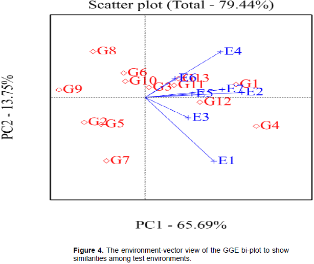
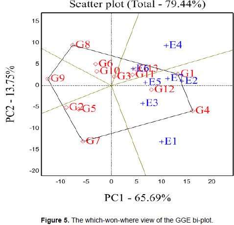
The GGE bi-plot used in this study constitutes a summed up of 74.99% total variance of the first two principal components. As indicated by Yan and Thinker (2006), the similarity between two environments as well as genotypes is determined by both the length of their vectors and the cosine of the angle between them (Figure 4). E1 is at about 90o with E4 and E6 indicating that it had no correlation with these environments and could produce less similar information about the tested genotypes (Figure 4). But the other environments had vectors that were linked with less than 90o, indicating, these environments were positively correlated with each other. E2 had longest vector and small IPCA2 and that was relatively the most representative and discriminating environment and considered as the ideal environment for generally adapted genotypes. Hence, Genotypes with above average yield in this environment had above average yield in all environments. E1 and E4 were the most discriminating but least representative environments which were with little information of the genotypes and favorable for specifically adapted genotypes. Exclusively, E6 was neither discriminating nor representative environment. To clearly display graphically, the 'which-won-where' pattern of a polygon view of GGE bi-plot is exhibited in Figure 5. The polygon was formed by connecting the vertex genotypes that were furthest away from the bi-plot origin such that all other genotypes were included in the polygon. From the polygon view of bi-plot analysis (Figure 5) the bi-plot showed there were two different sesame growing environments. The one environment includes the high yielding environments (E4 and E6), which were in the Dansha area with the winning genotype G1; the second environment contained the low to medium yielding environments (E1, E2, E3, E5 andE7), which were under Humeraand Sheraro areas with a vertex genotype G4. The other vertex genotypes (G7, G8 and G9) without any environment in their sectors were not the highest yielding genotypes at any environment rather they were the poorest genotypes of all or some environments.
CONCLUSION AND RECOMMENDATION
The combined ANOVA showed significant differences among the sesame genotypes in this study for meangrain yield across environments. The results also showed that the environments were highly variable with respect to climatic and/or edaphic factors. This GEI in turn indicated that, the performance or ranking of the genotypes was variable across environments and it was difficult to identify superior genotype for all environments or locations. The GGE bi-plot identified two sesame growing environments; the area of Dansha (E4 and E6) with G1 as a winning genotype, and the other environment encompassing Sheraro (E7) and Humera and Dansha (E1,E2, E3andE5) with G4 as a wining genotype.
The AMMI bi-plot and GGE bi-plot of grain yield data identified G12 as the most stable and widely adapted genotype for grain yield while, G4 and G1 were specifically adapted in the favorable environments.
The authors have not declared any conflict of interests.
REFERENCES
|
Ahmed MBS, Ahmed FA (2012). Genotype X season interaction and characters association of some Sesame (Sesamumindicum L.) genotypes under rain-fed conditions of Sudan. Afr. J. Plant Sci. 6(1):39-42.
|
|
|
|
Allard RW, Bradshaw AD (1964). Implication of genotype by environmental interaction in applied plant breeding. Crop Sci. 4(5):503-506.
Crossref
|
|
|
|
|
Buss J (2007). Sesame production in Nampula: Baselinesurvey report,
|
|
|
|
|
Ceccarelli S (2012). Plant breeding with farmers – a technical manual.ICARDA, Syria.
|
|
|
|
|
CSA (2013).Agricultural Sample Survey. Report on Area and Production, Volume III, Addis Ababa, Ethiopia.
|
|
|
|
|
FAOSTAT (2012).(Food and Agriculture Organization of the United Nations). Available at: http://faostat.fao.org/
|
|
|
|
|
GenStat (2009).GenStat for Windows (14th Edition) Introduction. VSN International, Hemel Hempstead.
|
|
|
|
|
Hagos T (2009). Genotype by Environment Interaction and yield stability of Sesame (Sesamum indicum L.) genotypes under North Western and Western lowland Tigray, M.Sc. thesis, Mekelle University, Ethiopia.
|
|
|
|
|
John A, Subbaraman N, Jebbaraj S (2001). Genotype by Environment Interaction in Sesame (Sesamum indicum L.): Sesame and safflower newsletter no. 16, Institute of Sustainable Agriculture, FAO, Rome.
|
|
|
|
|
Steel R, Torrie J (1980).Principles and Procedures of Statistics a Biometrical Approach. 2nd ed. McGraw-Hill, Inc. pp. 471-472.
|
|
|
|
|
Yan W (2001). GGE bi-plot windows application for graphical analysis of multi-environment trial data and other types of two-way data. Agron. J. 93:1111-1118.
Crossref
|
|
|
|
|
Yan W, Kang MS, Ma B, Woods S, Cornelius PL (2007). GGE bi-plot vs. AMMI analysis of genotype-by-environment data. Crop Sci. 47:643-653.
Crossref
|
|
|
|
|
Yan W, Thinker NA (2006). bi-plot analysis of multi-environment trial data: Principles and applications. Can. J. Plant Sci. 86:23-645.
Crossref
|
|
|
|
|
Zenebe M, Hussien M (2009). Study on Genotype X Environment Interaction of Oil Content in Sesame (Sesamum indicum L.). Middle-East J. Sci. Res. 4:100-104.
|
|
|
|
|
Zerihun J, Amsalu A, Fekadu F (2011). Assessment of yield stability and disease responses in Ethiopian Barley (Hordeium vulgare L.) Landraces and Crosses. Int. J. Agric. Res. 6:754-768.
Crossref
|
|
|
|
|
Zobel RW, Wright MJ, Gauch HG (1988). Statistical analysis of a yield trial. Agron. J. 80:388-393.
Crossref
|
|