Common bean (Phaseolus vulgaris L.) is one of the major sources of dietary proteins, vitamins, and minerals to millions of resource-poor farmers, particularly in developing countries (Broughton et al., 2003). Beans are the main grain legume crop grown in Tanzania, where they  are  often   intercropped  with  maize. Cultivation of beans can be seen in most areas of Tanzania (Hillocks et al., 2006).

In agricultural experimentation, a large number of genotypes are normally tested over a wide range of environments (locations, years, growing seasons, etc). Due to the variation of the climate, soil properties and the inherent potential of genotypes, crop yield may vary from one  environment  to  another  as  a  result  of  interaction between the environment and genotypes. The presence of a genotype x environment interaction automatically implies that the behavior of the genotypes depend upon the particular environment in which they are evaluated (Nchimbi-Ms and Tryphone, 2010). Therefore, it was important to study the genotype and environment interaction of the genotypes in order to identify high-yielding and stable cultivars and discriminating and representative test environments (Yan, 2001).

The genotype x environment interaction for certain bean characteristics, such as yield, may hinder cultivar recommendation for large geographical areas (De Araújo et al., 2003). The selection of genotypes to maximize yield when genotype rank changes occur across environments is complicated because of the complexity of genotype responses (da Silveira et al., 2013). A recently developed graphical data summary, called Genotypes main effects and Genotype x environment interaction effects (GGE) biplot, can aid in data exploration. GGE biplot is a Windows application that performs biplot analysis of two-way data that assume an entry × tester structure. A multi – environment trial data set, in which cultivars are entries and environments are testers, was used to demonstrate the functions of GGE biplot (Yan, 2001). These include but are not limited to: (i) ranking the cultivars based on their performance in any given environment, (ii) ranking the environments based on the relative performance of any given cultivar, (iii) comparing the performance of any pair of cultivars in different environments, (iv) identifying the best cultivar in each environment, (v) grouping the environments based on the best cultivars, (vi) evaluating the cultivars based on both average yield and stability, (vii) evaluating the environments based on both discriminating ability and representativeness, and (viii) visualizing all of these aspects for a subset of the data by removing some of the cultivars or environments. GGE biplot has been applied to visual analysis of genotype × environment data, genotype × trait data, genotype × marker data, and diallel cross data (Yan, 2001). GGE biplot identifies G x E interaction patterns of data and clearly shows which variety performs best in which environments and thus facilitates mega- environment identification (Gurmu, 2017; Shiri, 2013; Yan, 2001). Therefore, there is need for understanding the nature of G x E interaction, quantifying its magnitude and identifying stable and widely adapted common bean genotypes before release (Gurmu, 2017).

G x E due to different responses of genotypes in diverse environments, makes choosing the superior genotypes difficult in plant breeding programmes. Traditionally, plant breeders tend to select genotypes that show stable performance as defined by minimal G x E effects across a number of locations and/or years. The term   stability   is   sometimes   used   to   characterize  a genotype which shows a relatively constant yield independent of  changing  environmental  conditions.  On the basis of this idea, genotypes with a minimal variance for yield across different environments are considered stable (Kundy and Mkamilo, 2014). The current study was conducted to evaluate the G x E interaction for the plant yield of common bean genotypes in Kagera Region, in order to identify stable high yielding and stable genotypes.

 

Experimental sites and Materials used for the study

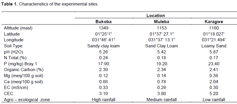
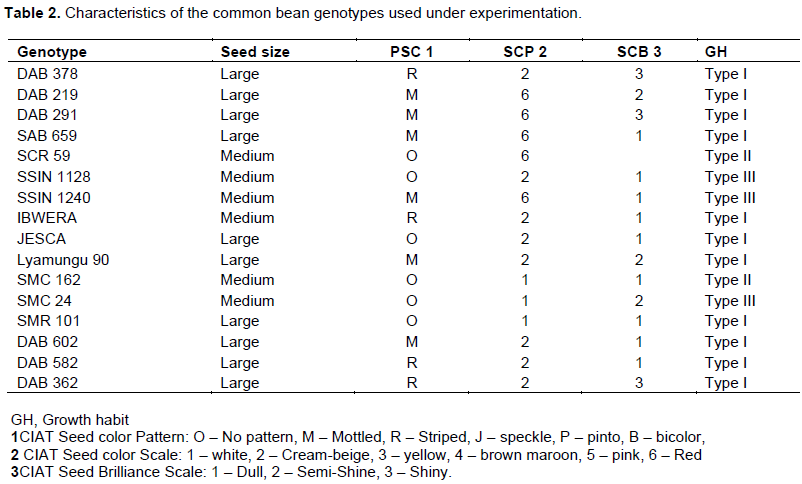
The study was conducted during 2017/2018 cropping season in three different agro ecological sites of Kagera Region which includes Bukoba, Karagwe and Muleba Districts (Table 1) where farmers grow common beans as food and commercial crop as well. A total of 16 common bean genotypes, 13 introduced genotypes from the International Center for Tropical Agriculture CIAT, two released varieties (Lyamungu 90 and JESCA as control) and one landrace (Ibwera as local check) were used during the experimentation  across three environments. The list of these genotypes is presented in Table 2.

 

 

 

Experimental design and field layout

The experiment was laid out in Randomized Complete Block Design (RCBD) arranged in a split plot layout with three replications in each site (Table 1). Two factors were used; the first was location (the main factor), three Districts of Kagera Region (Bukoba, Karagwe and Muleba) with different agro climate was involved during the experiment. The second factor was genotypes (the sub factor): sixteen common bean genotypes were used in the experiment. The experimental unit size was 3 by 1.5 m, consisting of four rows; spacing was 50 cm between rows and 20 cm with row, two seeds per hill. Hand- hoe weeding and fertilizer application were done twice when beans had one trifoliate leaf and before flowering. Fertilizer used was NPK: 20:10:10 at recommended rate. All recommended agronomic practices for common bean productions were followed.

Statistical model

y_ijk = µ + α_i + β_j + (αβ)_ij + c_ik + e_ijk                                                    (1)

Where

µ is a population mean.

α_i is the main effect of location (A).

β_j is a main effect of genotypes (B)

(αβ)_ij  is the interaction effect of A and B

c_ik is the plot error distribution, k = 1, 2.

e_ijkis the sub – plot  error distribution, k = 1, 2.

Data collection

Days to 50% flowering (DF)

This was measured in days-after-planting and coinciding with the initiation of developmental stage R6 when 50% of the plants have one  or  more  flowers  (Schoonhoven  and  Pastor-Corrales, 1987).

Days to physiological maturity (DPM)

This  was  measured  in  days-after-planting and coinciding with the initiation of developmental stage R9 when 50%of the plants have reached physiological maturity (Schoonhoven and Pastor-Corrales, 1987).

Number of pods/plant

Number of pods per plant were recorded from ten plant selected randomly in the net plot and the average of the plot was  calculated.

Number of seeds/pod

The  number  of  seed  per  pod  was  recorded  from  ten  randomly selected pods in the net plot and the average of the plot was calculated.

Seeds size

Seed size is expressed as the weight in grams of 100 randomly chosen seeds and categorized as follows; Small: Less than 25 g, Medium: 25 g to 40 g, Large: More than 40 g (Schoonhoven and Pastor-Corrales, 1987.

Grain yield (kg/ha)

Harvesting  was  done  for  two  middle  rows of each plot and grain yield was adjusted by converting plot yield (at 14% moisture content) to seed yield per hectare (Kadhem and Baktash, 2016).

Statistical analysis

The additive main effect and multiplicative interaction Analysis

The data for grain yield were pooled to perform the analysis of variance across the environment. Since the pooled analysis of variance considers only the main effects, the additive main effect and multiplicative interaction model (AMMI) was computed using Genstat software. The AMMI analysis is a combination of analysis of variance (ANOVA) and principal component analysis (PCA) in which the sources of variability in genotype by environment interaction are partitioned by PCA (Ana et al., 2011).

The main idea of the AMMI models is: (i) first apply the additive of the variance model (ANOVA) to a two-way table and (ii) secondly apply the multiplicative PCA model to the residual from the additive model (Gauch, 1992). The AMMI model with multiplicative terms can be written as:

Y_ij = µ + G_i + E_j +Σ_k=1λ_kγ_ik α_jk + ρ_ij + ε_ij                                                                      (2)

Where: Yij is the yield of genotype i in environment j; µ Grand mean; G_i the genotype means deviations (the genotype means minus the grand mean); E_j the environment mean deviations; λ_k the singular value for the PCA axis k; γ_ik and γ_ik α_jk are the genotype and environment PCA scores for PCA axis k; K is the number of PCA axes (Kadhem and Baktash, 2016).

The AMMI model was used to identify genotypes(s) which are adapted in different environment. The AMMI’s stability values (ASV) were computed using Equation 3.

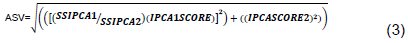
Where SSIPCA1/SSIPCA2 is the weight given to the IPCA1 value by dividing the IPCA1 SS by the IPCA1 SS; and the IPCA1 and IPCA2 scores are the genotypic scores in the AMMI model (Rad et al., 2013).

Genotype and genotype by environment (GGE) – Biplot analysis

The GGE biplot methodology was used to analyze the multi - location genotype yield trial data to evaluate the grain yield stability and identify superior genotypes using  the  GenStat  v.13  software. GGE biplot analysis was also used to generate graphs for: (i) comparing environments to the ideal environment; (ii) the “which-won-where” pattern; (iii) environment vectors. The angles between environment vectors were used to judge correlations (similarities/dissimilarities) between pairs of environments (Shiri, 2013).

 

 

Analysis of variance

The single site analysis of variances (Table 3) revealed the high significance differences among the genotypes in each tested environment but the results shows variability of the genotype rank from one environment to another, this justifying the conduction of a more refined analysis so that to increase the efficiency of the selection and indication of cultivars. In this sense, AMMI analysis represents a potential tool that can be used to deepen the understanding of factors involved in the manifestation of the G × E interaction (da Silveira et al., 2013).

 

 

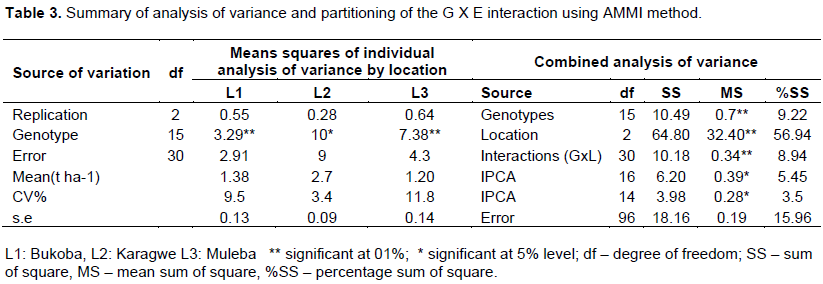
The analysis of variance of the AMMI model indicated that environments accounted for 56.9% of the total sum of square; genotypes effect explained 9.2% and the G x E interaction effect accounted 8.9% for the 16 genotypes tested across three environments (Table 3) and were all significant (P < 0.01). A large SS for environments indicated that the environments were diverse, with large differences among environmental means causing most of the variation (da Silveira et al., 2013) in genotype grain yield. This means there were large environmental effects on the genotypes performance across the environments than the interaction between the genotypes and the environment.

Mean performance of the genotypes in each and across environments

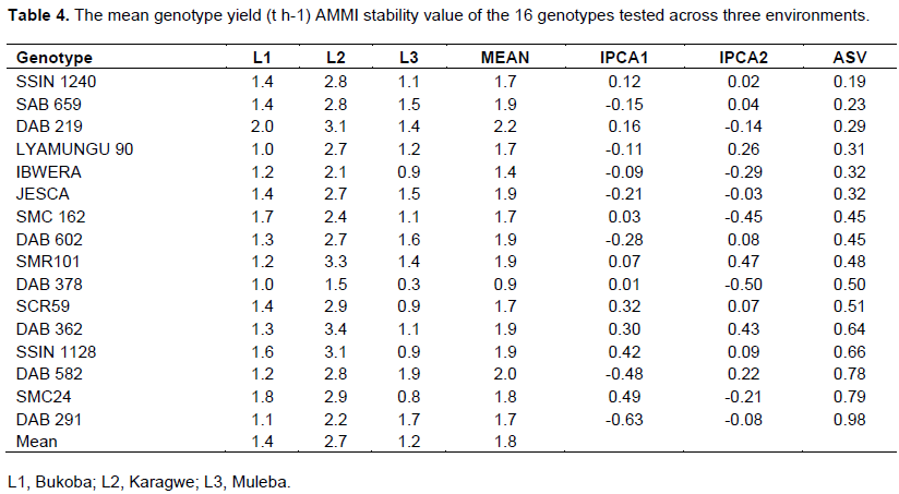
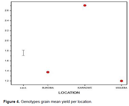
The mean grain yield of the genotypes as presented in Table 4.  Karagwe  site (L2) was the best environment for common bean production that gave the average grain yield of 2.7 t ha^-1, followed by Bukoba which gave 1.38 t ha^-1 and Muleba was the least with an average production of 1.20 t ha^-1 (Table 4). In Karagwe, plant responded vigorously and most of the genotypes performed more than 2 t ha^-1 with high scores of the plant vigor of scale 1 and 2 to most of the tested genotypes, while in Muleba which is the least site in the performances of the genotypes was poor with some of the genotypes scores plant vigor of scale 3 (good) and scale 5 (intermediate) according to Schoonhoven  and  Pastor-Corrales, 1987.

 

 

AMMI’s stability values (ASV)

The ASV is the distance from zero in a two dimensional scatter gram of IPCA1 (interaction principal component analysis axis 1) scores against IPCA2 scores. Since the IPCA1 score contributes more to GE sum of scores, it has to be weighted by the proportional difference between IPCA1 and IPCA2 scores to compensate for the relative contribution of IPCA1 and IPCA2 total GE sum of squares. From the calculation of Equation 1, genotypes SSIN 1240, SAB 659, DAB 219 and Lyamungu 90 had shown higher adaptive capacity compared to others genotypes due to their lower AMMI stability values as shown in Table 4 as described by Al-Naggar et al., 2018, that a genotype with least ASV and IPCA scores (either negative or positive) are considered as the most stable while the genotypes SSIN 1128, DAB 582, SMC24 and DAB 291 had shown lesser adaptive capacity.

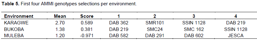
Some  of  the  genotypes   may  perform  better  in  one environment but the same genotype performs less in the other environment. For instance, the genotype DAB 362 ranked number one in performance with average yield of 3.363 t ha^-1 in Karagwe site but it did less in other two environments, like – wise DAB 219 ranked number one in Bukoba and in Karagwe ranked number four but in Muleba it did not appeared in top four performed genotypes (Tables 4 and 5). As stated by Kadhem and Baktash (2016) the best genotype needs to combine good grain yield and stable performance across a range of production environments. In this study only two genotypes DAB 219 and SSIN 1128 appeared to perform well in Karagwe and Bukoba sites. This happened despite the fact that the environments were diverse and caused for a great variation in grain yield which is quantitative trait, so the environmental factors are crucial determinant of yield expression (Kadhem and Baktash, 2016). However, the AMMI stability values revealed that SSIN 1240, SAB 659, DAB 219 were the most stable genotypes across three tested environments above checks which were Lyamungu 90, JESCA (released varieties) and Ibwera (landrace). Among them DAB 219 (arranged in increasing order of stability) had environment average yield of 2.169 t ha^-1 higher than any  tested genotypes (Table 4), while the first two more stable genotypes SSIN 1240, SAB 659 had environmental average yield of 1.737 and 1.892 t ha^-1 respectively.

 

 

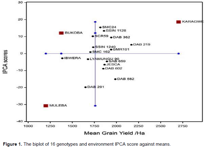
In biplot the differences among genotypes in terms of direction and magnitude along  the  X-axis  (yield)  and  Y axis (IPCA 1 scores) are important (Kadhem and Baktash, 2016). In the biplot display, genotypes or environments that appear almost on a perpendicular line of the graph had similar mean yields and those that fall almost on a horizontal line had similar interaction (Alberts, 2004). Genotypes or environments on the right side of the midpoint of the perpendicular line have higher yields than those on the left side. The score and sign of IPCA1 reflect the magnitude of the contribution of both genotypes and environments to GEI, where values closer to the origin of the axis (IPCA1) provide a smaller contribution to the interaction than those that are further away (characteristic of stability), whereas higher score (absolute value) considered as unstable and specific adapted to certain environment (Psychometrika, 1968; da Silveira et al., 2013). The characterization of each promising lines (genotypes) to mean grain yield and contribution  to  GEI  by  mean  of  IPCA1 (Alberts,  2004) based on these attributes our study  indicates that genotypes SMR 101, DAB 362, SSIN 1128, SMC 24 and DAB 219 were specifically adapted to Karagwe which was the high yielding environment as shown in Figure 2.

The genotypes SSIN 1240, SAB 659 and DAB 219, SMR 101, SMC 162, IBWERA, Lyamungu 90, JESCA and DAB 602 showed greater stability with the average closer to the overall average of the tested genotypes. However, genotypes SSIN 1240, SMC 162, IBWERA and Lyamungu90 were identified to be adapted to low yielding environment since they appeared on the left side of the mid-point representing grand mean in Figure 1. The GGE analysis was performed on the average grain yield of the 16 common beans genotypes tested in three different sites. The results showed that the GGE biplot explained 89.5% of the genotype main effects and the Genotype by Environment interaction. The primary (PC1) and Secondary (PC2) components explained  59.8 and 29.8% of the genotypes main effects and G x E interaction respectively (Figure 2). The genotypic PC1 scores greater than zero classified the high yielding genotypes while PC1 scores less than zero identified low yielding genotypes, unlike genotypic PC1, genotypic PC2, scores near zero showed stable genotypes whereas large PC2 scores discriminated the unstable ones (Jalata, 2011).

 

 

 

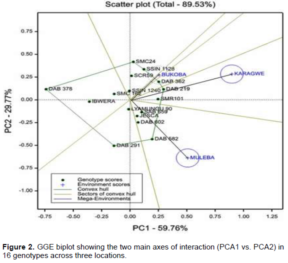
The plot of PCA1 vs. PCA2 revealed that SSIN 1240, SAB 659, DAB 219 and Lyamungu 90 were the most stable genotypes due to the fact that, they were found closer or at a lesser distance from the center of the biplot when compared with other genotypes, while SSIN 1128, DAB 582, SMC24 and DAB 291 were considered as most unstable genotypes among all other tested genotypes across three environments as shown in Figure 2, similar result was also reported by Kadhem and Baktash (2016).

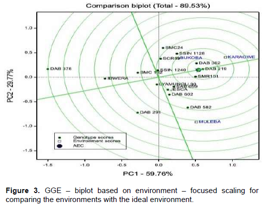
The GGE biplot was also used to show the association among the tested environment. Figure 2 show that Karagwe and Muleba exhibits longer vectors compared to Bukoba this contributed more to the environment sum of square as also indicated in the ANOVA table (Table 3). Genotypes and environments positioned close to each other in the biplot have positive associations, thus these enable the creation of agronomic zones with relative ease (Alberts, 2004). In the current study, the polygon  view  of GGE biplot for grain yield indicates the best genotype(s) for each environment(s). In Figure 3 the genotypes SMC 24, SSIN 1128, DAB 362, Dab 219, DAB 582, DAB 291 and DAB 378 were the best or poorest genotypes because they are located on the vertex of a polygon (Hagos and Abay, 2013).

 

 

The vector view of  GGE-biplot (Figure 2) provides a succinct summary of the interrelationships among the environments; all environments were positive correlated because all angles among them were smaller than 90° (Rad et al., 2013). The correlation between Karagwe and Bukoba is stronger than that of Muleba and either of the other two locations. The results suggesting that indirect selection for grain yield can be practical across the tested environment, this means adaptable genotypes in Karagwe may also show a similar respond in Bukoba and less response in Muleba.

The GGE biplot was also used to draw the polygon for G × E interaction effect from which different interpretations can be derived. The polygon is formed by connecting the markers of the genotypes that were further away from the biplot origin such that all other genotypes were contained in the polygon as shown in Figure 2. The polygon view of a biplot is the best way to visualize the patterns  of  interaction  between  genotypes and environments, and to effectively interpret a biplot (Shiri, 2013).

An environment is more desirable if it is located closer to the ideal environment. Thus, using the ideal environment as the centre, concentric circles were drawn to help visualize the distance between each environment and the ideal  environment  (Yan  et  al.,  2000;  Yan  and Rajcan, 2002). Figure 3 shows that Karagwe was an ideal test environment in terms of being the most representative of the overall environment. The graphical representation of the means performances of the genotypes per location which indicates that, Karagwe is better performing environment (Figure 4).  However, the vector of  GGE-biplot  shows  interrelation  among  tested environment in which all three environments were positive correlated and the GGE – biplot, for comparing environments with ideal environment, positioned Karagwe site at the center of the concentric circles (Figure 3). As stated by da Silveira et al. (2013) genotypes and environments positioned close to each other in the biplot have positive associations, thus these enable the creation of agronomic zones with relative ease. Both the genotype and the environment determine the phenotype of an individual. The effects of these two factors, however, are not always additive because of the interaction between them. The large G x E variation usually impairs the accuracy of yield estimation and reduces the relationship between genotypic and phenotypic values (Ssemakula and Dixon, 2007).  

 

 

 

 

 

 

 

 

 

The results of this study indicates the significant genotypes environment interaction in grain yield across the tested environments, this means each genotype responded differently when exposed to different location due to variations in climate and edaphic factors. It was difficult to identify genotype which was superior for all tested environment. Therefore, based on GGE and AMMI multivariate analyses which performed evaluation of genotypes adaptability/stability across the tested sites, genotypes DAB 362, and SMR 101 could be recommended to be used in Karagwe. While genotypes SMC 24, SMC 162 and SSIN 1128 could be used in Bukoba, likewise genotypes DAB 582, DAB 602 and DAB 291 could be used in Muleba. SSIN 1128 and DAB 219 could be grown in Karagwe as well as in Bukoba.

 

The authors have not declared any conflict of interests.