Pipelines experience integrity deterioration due to natural causes, operating conditions and poor maintenance which may lead to the formation of irregularities on the inner surface of said pipelines and pitting problems.  There are several causes which can cause the formation of irregularities such as spillages of soldering flux inside the pipe during welding processes and erosion by foreign particles. Improper joints and bends of pipes can also  be the cause of irregularities. Irregularities can also be formed due to high fluids velocities flowing in the pipes which basically will scour the pipes’ walls and subsequently would lead to the formation of localised corrosion (Hayes, 2011; Tan et al., 2020). Irregularities such as dents, scratches and bumps inside pipelines will force fluids to flow into other smooth inner surface pipes with  velocities  different  from their initial values. This can cause a turbulence flow in the pipelines especially of smaller flow area. Many approaches have been taken to overcome this problem such as the introduction of smart pipe inspection gauge (PIG). However, the smart PIG is not suitable for all pipelines. Since most of the pipelines consist of sharp bends, reduced port valves and loops can cause problems for the smart PIG’s operational inspections, that is, it can get stuck in the middle of pipelines during operations. When a smart PIG gets stuck, the whole operation must be shut down in order to retrieve the instrument. This will result in non-production time and unnecessarily increase the operational cost (Meisner and Leffler, 2006).

Tomography has been widely applied in various kinds of fields such as medical, engineering, biotechnology, etc.  Tomography is a process of imaging by sectioning interior solid materials from the outside using waves of energy without affecting the object. Process tomography can give real-time cross-sectional images inside the materials (Martin et al., 2001; Qureshi et al., 2021). A 2-D or 3-D image of some physical quantity inside the object can be obtained using external sensors to detect signals from the boundaries of the object (Dickin and Hoyle, 1992; Schlaberg et al., 1997; Takiguchi, 2019).  The measurements variables are usually temperature, pressure, power level, component geometry, etc. (Dickin and Hoyle, 1992). There are three basic elements in tomography process including sensor, electronic circuit, and image reconstruction system. Sensor is the most important element as it interrogates the process and information obtained from the process will affect the accuracy of the whole system (Dickin and Hoyle, 1992; Almutairi et al., 2020).

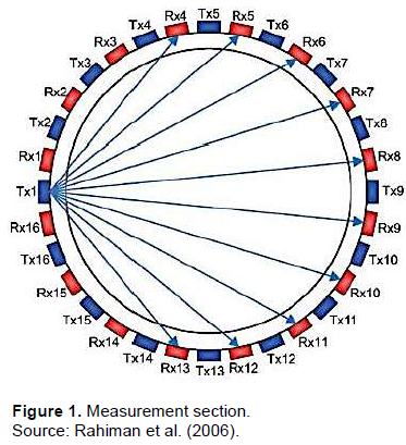
Ultrasonic tomography is commonly used in the oil and gas industry for monitoring irregularities inside the pipe as it can locate and visualise the presence of irregularities inside the pipe (Mudali et al., 2006; Zaman et al., 2020). Ultrasonic tomography is a non-invasive technique, in which the sensors are mounted outside the pipe to be tested without making any changes to it and it does not interfere with the processes inside the pipe during operation. This technique can give accurate results, and is an environmental-friendly method (Takiguchi, 2019). The ultrasonic signal is transmitted from the transmitter and propagated along the tested material. The signal will be received by the receiver and sent to the Data Acquisition System (DAS) for analyses. The result is in image form after being processed in an image reconstruction system. The ultrasonic sensors can be divided into transmission-mode, reflection-mode, and emission-mode. These modes are based on the change of physical properties of the transmitted signals. There will be changes of output voltage when there are obstructions in the ultrasonic path length, which indicates that the absorption of ultrasonic signals has occurred (Abdul Rahim et al., 2007; Lowe et al., 2020). Ultrasonic sensors   were   mounted   around   the   surface   of   the targeted vessel as shown in Figure 1 and based on the figures Tx and Rx which represent the transmitter and receiver, respectively.

Pipe surface preparation must be done very carefully so that the original curvature of the pipe could be preserved.  The transducer and pipe were positioned in parallel axis because one-degree error could cause one percent change in path length. A coupling was used to provide more reliable transmissions of the ultrasound waves between the pipe wall and transducers. Coupling creates a free-air region between the transducer and pipe wall. The waves will scatter when they pass through the air and the transmitted signal will never pass through the pipe (Rahiman et al., 2006; Lee et al., 2010; Lowe et al., 2020).

The purpose of this paper is to demonstrate development of an ultrasonic instrumentation system which can monitor and detect any irregularities inside a pipe.

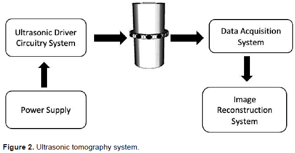
An ultrasonic tomography system consists of three main parts, which are a sensor unit, a Data Acquisition System (DAS) and an Image Reconstruction System as shown in Figure 2. The sensors’ arrangement was designed to interrogate the sensing area from various viewing angles. The ultrasonic signal that was transmitted from the transmitter is propagated through the tested pipe; thereafter, the ultrasonic signal was received by the receiver and sent to the data acquisition system (DAS) to obtain data from the tested pipe. For this project, the DAS acquired raw measurements from the ultrasonic sensor. The DAS’ outputs were sent to the image reconstruction system to get the image results.

Rig design

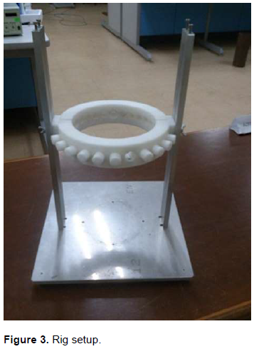
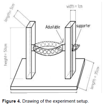
The rig was designed based on the tomography system concept, where ultrasonic sensors were mounted on the outside of the pipe for inspection. In order to mount the sensors circling the tested pipe, sensors in the shape of circular rings were used. There were three major parts in designing the rig to accomplish the intended experimental works, namely the square base, circle ring sensor unit, and ring holder. The dimension of the base was 35 cm x 35 cm in a square shape.  The base was designed to hold the  ring  holder which is attached directly to it using screws. The circle ring was attached to its holder using a butterfly screw. This butterfly screw is adjustable and can be moved up and down depending on the position of the test pipe. The dimension of the ring holder was 1 cm x 5 cm x 50 cm in a rectangular shape. It was responsible to hold the circle ring of the sensor unit in a steady position during the experiment. The ring holder was designed to have a trail path with the length of 35 cm along it. The material used for the square base and ring holder was aluminium. Aluminium has a high resistance to corrosion and will not easily rust at room temperature. It can be stored in a laboratory without requiring any corrosion protection and can be used for long periods of time. The material used for the circle ring was Duracon. Figures 3 and 4 show the setup of the rig and drawing of the rig with exact dimensions respectively.

Design configuration of the ultrasonic tomography system

The system  was  designed  for  detecting  irregularities in a pipe. In the system, transmission-mode ultrasonic sensors were used, and these sensors were arranged to surround the metal pipe. When the transmitters transmitted signals through the test pipe, it was received by the receiver. The percentage of the received signal depended on the signals that managed to pass through the material. From the receiver, the information was transferred to the data acquisition system. The output of the signal was shown in voltage form. There would be a difference in the signal amplitude if there were irregularities detected in the pipe. A set of data obtained could then be processed using the image reconstruction system. The data was converted into images to investigate the inner conditions of the pipe.  It is important to arrange the sensors around the pipe so that the signal could cover every internal part of the pipe. In the transmission mode, the propagation of ultrasonic waves from the transmitter to the receiver was direct. Twelve transmitters and 12 receivers were attached to the ring holder, in which Tx represents the transmitter and Rx represents the receiver. The size of the ring holder must fit the test pipe so that there would be no air gap between the sensors and the pipe wall.  

The transmitter and receiver were placed in opposite directions. In this arrangement, the ultrasonic signals from transmitters propagated directly to the receivers. All the sensors were fitted into the hole at the ring holder which clamped around to the test pipe. It is imperative to note that the percentage of the received signal that could pass through the said pipe material was affected by the intensity of the signals. From the receiver, the information inside the test pipe was transferred to the data acquisition system. In this experiment, 12 sensors were used, consisting of 12 transmitters and 12 receivers.

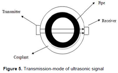
For the study, the transmission mode was applied, where two types of sensors were used, the transmitters and receivers. The sensors   were  placed  at  the  opposite  direction  surrounding  the tested pipe as shown in Figure 5. It was important to ensure that the transmitted ultrasonic signals could travel through the material tested because each material has different acoustic impedance. The ultrasonic signals were able to travel through different materials when there were no big differences in acoustic impedance between them. Acoustic impedance can be defined as the product of density of the material and its velocity (Tole, 2005; Laugier and Guillaume, 2010). This characteristic plays an important role in determining whether the ultrasonic signals transmitted by the transmitters can be received by the receiver. If there are big differences of acoustic impedance between the materials the signals travel through, the signal might not pass through the material. Hence, the signals will be reflected back to the transmitter (Stocksley, 2001).

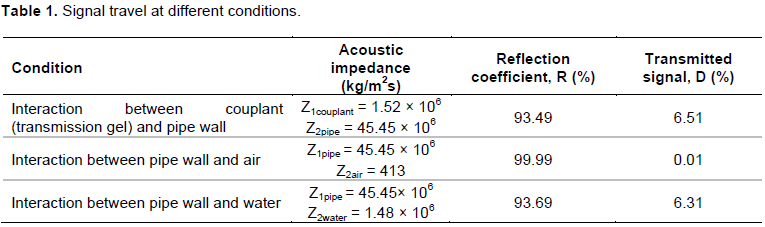
Three conditions were considered to simulate the number of signals that were able to reach the receiver. These included interaction between couplant and the pipe wall, interaction between pipe wall and air and interaction between pipe wall and water. Since the transmission mode was used in the experiment, it was necessary to make sure the signals could transmit through the material. In that case, the receiver must be able to receive the signals, and then acquire the data.  In order to make sure the signals can reach the receiver; a reflection coefficient has been introduced as shown in Equation 1.

where   Z₁ = acoustic impedance of the first material signal travelling

            Z₂ = acoustic impedance of the second material signal travelling.

The reflection coefficient is usually performed in terms of percentage. The total of the transmitted and reflected signals is 100%. So, to get the percentage of transmitted signals, a hundred must be subtracted by the reflected coefficient. This equation was applied to three conditions with an assumption that there is no energy lost while the signal travels along the path to the receiver as highlighted in Table 1. Based on the table, when air exists in the path of the travelling energy, almost all of the signals were reflected back to the transmitter. The existence of air in the pipe during the experiment must be avoided. A very small amount of transmitted energy to the receiver can be neglected since there will be losses of energy along the signal path.

Attenuation of the wave

Attenuation of wave is the reduction of energy and amplitude whenever waves travel along a certain distance. Every material has its own attenuation coefficient, and this will determine the energy loss when signals pass through it and can be calculated using Equation 2 (Peter et al., 2010).

where P_x = attenuation at the certain distance; P_o = initial pressure; α = attenuation coefficient; x = distance the signal travel.

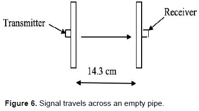
Equation 2 is applied in order to determine the energy losses when the signal travels through a test pipe. The signal travels across the pipe material and air. The travel distance of the signal was equal to the diameter of the pipe.  Figure 6 shows the signal’s travel path across an empty pipe and the signal lost was 81% when it travelled through the air (α_air = 0.00142 mm^-1) at the designed distance of 14.3 cm. This was due to the absorption of wave by air and pipe material. However, when waves travelled through water, about 65.7% energy was lost from the incident signal (Peter et al., 2010). The rest of the signals were received by the receiver.

Selection of the pipe and sensor

A steel pipe was used in this project due to availability and based on the utility pipes that we use in our daily life.  The size of the pipe used was 5” (143 mm). The length of the pipe was thirty (30) cm. The size of the pipe for the experiment was based on its small scale since the experiment was carried out in a laboratory. The size of the pipe indicated the number of sensors to be used. In this study, twenty-four sensors were used, consisting of twelve transmitters and twelve receivers. The sensors were used in order to get a detailed condition of the pipe.

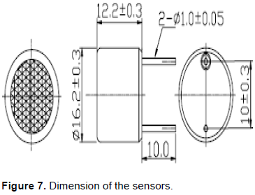
The sensors used in the experiment were the Ultrasonic Sensor EFC16T/R-2. These sensors have a frequency of 40 kHz and are based on transmission mode. The existence  of  air along  the  path can cause a large mismatch of acoustic impedance. The signal cannot pass through two mediums that have a large difference of impedance. Precaution steps must be taken, such as the use of couplant between sensors and the tested pipe in order to minimize the effect of air to the ultrasonic signals. The sensors functioned based on the interruption of sound waves due to objects detected in the path between the transmitter and the receiver. The strength of the signal received by the receivers was totally dependent on the alignment of the transmitter and the receiver. Table 2 shows the specifications of the sensors used for testing.

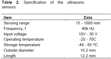
Figure 7 shows the actual dimensions of the sensors. Selection of the sensors is also important to ensure it fitted into the hole at the circle ring of the sensor unit which was 20 mm in diameter. The sensors were driven by an electronic circuit so it could operate based on its functions. Both the transmitter and the receiver have different types of circuits because both have different functions.

Pipe specimen preparation

Clay was attached to the pipe internal wall to represent the irregularities. Three different cases were carried out in the experiment by manipulating the amount of clay used to simulate irregularities which low, medium and heavy irregularities as shown in Figure 8.

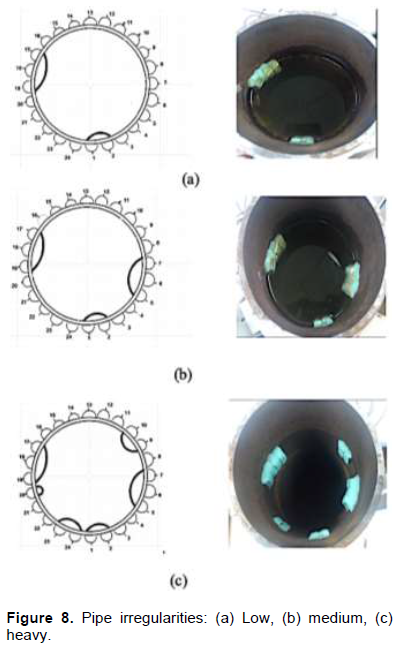
The degree of irregularities was set based on the degree of spread of the pasted clay on the pipe. The more the clay was spread, the heavier the irregularities. The pipe was divided into 24 sections and marked with respective numbers. Since the transmitter and the receiver were placed in opposite positions to each other, position 1 was marked Tx1 for the transmitter and the opposite position was marked Rx1 for the receiver. For the second position, it was marked Tx2 for the transmitter and Rx2 for the receiver. This process was repeated until Tx12 and Rx12 (Figure 9). This made it easier  to  determine  the position of irregularities when constructing the tomography images. Water was used as the medium for the ultrasonic signals to propagate from the transmitter to the receiver.

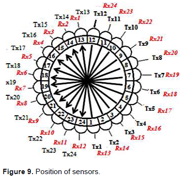
Image reconstruction

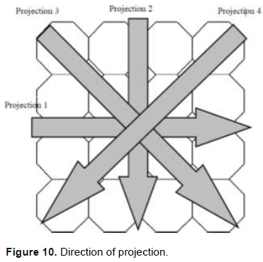
All data recorded from the three cases were processed using MATLAB software to produce 2-D tomography images. The images represented the actual conditions inside the tested steel pipe.  The images consisted of several colours in order to differentiate between the clean parts and the irregularities present inside the pipe, which were blue and red colour respectively. From the colour on the images, the positions of simulated irregularities were determined inside the pipe. The image was reconstructed based on the number of projections to be investigated. Figure 10 shows the direction of projections.

Experimental setup

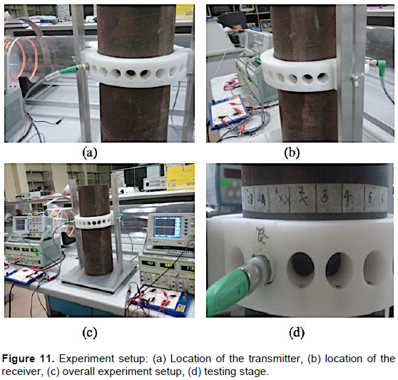
Figure 11 shows the experiment setup. In the experiment, the steel pipe was placed in the ring which was supported by an aluminium supporter. The steel pipe must be held steadily to ensure the ring would not move up or down. It was to ensure that  the  alignment  of the sensor was precise. In that way, the ultrasonic signals from the transmitter could reach the receiver as much as possible.

40 kHz ultrasonic sensor testing

The ultrasonic sensors used in the development of the ultrasonic tomographic instrumentation system were EFC16T/R-2 with a frequency of 40 kHz. Testing of the ultrasonic sensors was carried out to check the capabilities of the sensors by observing responses of ultrasonic signals through different mediums. The distance between transmitter and receiver was set at 10 cm. The changes of the ultrasonic signal were observed using HAKO FX-952 oscilloscope. The transmitter and receiver circuit (Courtesy Kerry D. Wong) were built using the EAGLE software in order to operate the sensors.

The testing was carried out in open air, to observe whether the ultrasonic signals could be transmitted through open air or otherwise. The input signals from the ultrasonic transmitter sensor were shown to be at the lower response that was blue in colour. The output of the ultrasonic signals in yellow indicated no response because the air reflected the waves, causing it to scatter to the surroundings. This was due to air having the lowest acoustic impedance value. Based on the calculation, the existence of air in the travel path of the ultrasonic signals caused almost 99.99% of the signals to be reflected and thus, not being able to reach the receivers. This was due to the big difference of acoustic impedance along the path. Therefore, the existence of air in pipes during experiments must be avoided. Similar results were obtained by Fazalul Rahiman et al. (2008) who used water/gas as a medium, proving that 99.94% of ultrasonic signals were reflected at the liquid/gas boundary and liquid region only when large different acoustic impedance existed between the gas and liquid mediums. The small amount of remaining ultrasonic signals that managed to pass through the water/gas medium was not able to reach the receiver because it experienced losses of energy during its journey along the ultrasonic path. It can be concluded that ultrasonic signals were detectable when there was no gas in the ultrasonic signal travelling path.

The second test was carried out to investigate the output response of ultrasonic signals when the signals travelled through the steel plate. The ultrasonic sensor was placed as close as possible to the plate, to avoid any air existence that could interrupt the propagation of ultrasonic signals. Three similar steel plates were used to observe the output response. The couplant was placed on the plate to equilibrate the acoustic impedance between the ultrasonic sensor and the plate. In that way, the ultrasonic signals were able to travel through the plate from the transmitter to the receiver. A similar testing was done based on two and three plates. The oscilloscope used in the experiment was set to give a high voltage value when the ultrasonic signal was absorbed by the material along its propagating path. The ultrasonic signal responses changed when a different plate thickness was used for the testing. The difference in value increased when the plate thickness increased. The principle applies to this experiment since simulated irregularities caused the difference of thicknesses in the pipe wall. Data interpreted from the ultrasonic output response was based on the difference of the low peak signals and the high peak signals.

Irregularities observation

Readings were collected in voltage. Figure 12 shows the voltage value obtained at all sensors, that is, reading between 2.1333 to 3.1333 V and 5.4677 to 7.5333 V when the ultrasonic signals passed through clean and irregularities pipe, respectively.

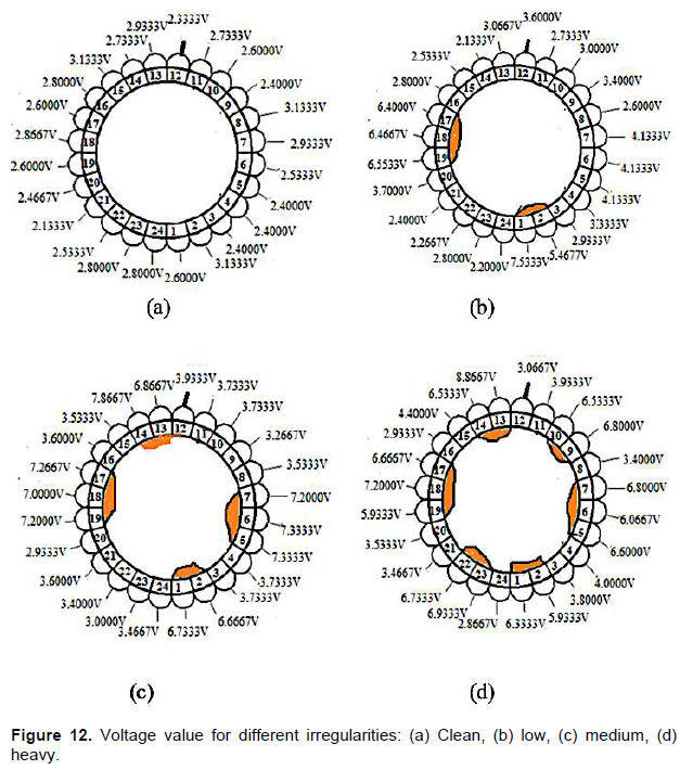
For clean pipe, the ultrasonic signals travelled from the transmitter  to  the  receiver without any interference from irregularities. Absorption of ultrasonic signals did not occur when the signals travelled through the pipe. Inconsistency of data obtained for the clean pipe experiment was due to the stability of the ultrasonic signal. Ultrasonic signals were unstable because they might be affected by surrounding factors. The ultrasonic waves changed rapidly during the experiment and caused variation of the output data.

A similar situation occurred when the experiments for low, medium, and high irregularities were carried out.  Nevertheless, the output data for the clean pipe was still within the low range value which could be distinguished from the pipes with irregularities that had high voltage value ranges. Another factor that could contribute to the inconsistency of output data was the presence of noise while carrying out the experiment. Based on the principle, noise is divided into two different categories, namely acoustic and non-acoustic noises. Acoustic noise usually comes from the material structure noise. Meanwhile, non-acoustic noise is subjected to electrical circuit noise and pulse noise, which is also known as instrumentation noise. The presence of these noises which cause the signal instability would lead to the variation of the final output (Chen, 1998).

For irregularities, the oscilloscope used in the experiment gave a high voltage value when the signals travelled through any irregularities. Absorption of ultrasonic waves occurred when it travelled through clay. Absorption phenomenon occurred, causing the ultrasonic waves to attenuate, losing energy during the propagation along the path from the transmitter to the receiver. Every material  has  a  different   attenuation   coefficient   which determines how much ultrasonic waves can be absorbed (Peter et al., 2010). The highlighted column represents the existence of irregularities inside the pipe, while the rest are clean parts. Therefore, if there was any absorption of the ultrasonic signals, the value of the output voltage would increase.

Image of irregularities

Figure 13 shows all the image of the irregularities of the tested pipe specimen. The image generated for the clean pipe showed that there were no irregularities present inside the pipe.  The blue colour in the image indicated water and there were no irregularities detected by the ultrasonic signals. The  image  generated from the Matlab software showed that most of the pipe’s inner area was blue in colour and corresponds with the data collection in Figure 12.

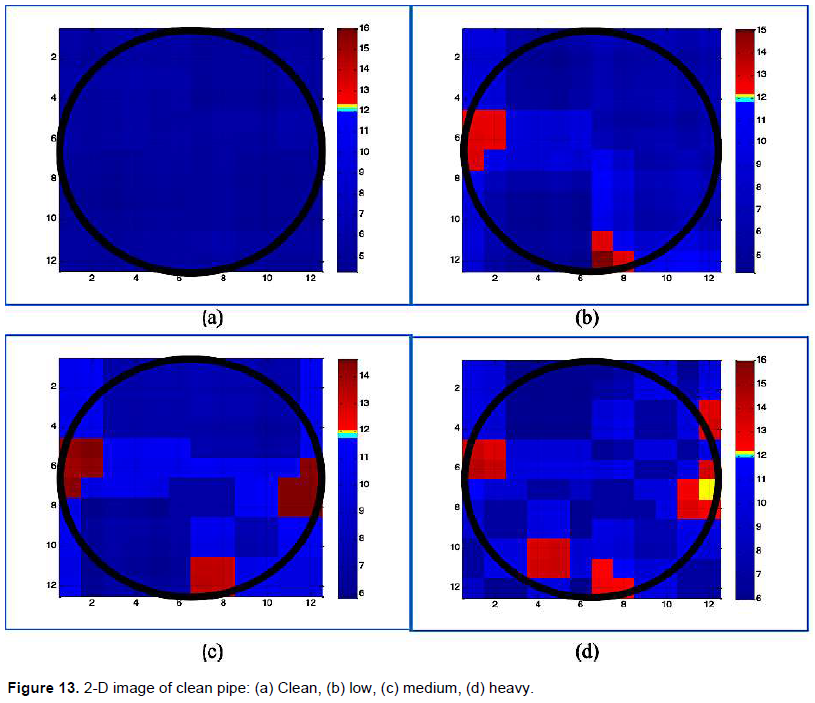
For the presence of irregularities inside the pipe, it can be observed that two different colours appeared in the images, which were blue and red. The red colour represented simulated irregularities at the wall of the pipe. The position of simulated irregularities in the reconstructed image showed synchronization with the real pipe. The different colour in the image indicated that there were obvious differences in voltage values due to the presence of irregularities.

The capability of ultrasonic tomography to visualise the internal conditions of the pipe had been proven by Rahiman et al. (2014) which was based on the time-flight and arrival-time of ultrasonic  signals from  the transmitter and the receiver.  On the other hand, this project’s output data was observed from the difference responses of the ultrasonic signals in terms of amplitude when it travelled through different mediums. These two approaches were proven to be able to give real visualisations of the tested pipe. However, environmental factors had caused instability of the ultrasonic signals while it propagated from the transmitter to the receiver such as the presence of noise and acoustic noise from the ultrasonic sensors circuit as well as discontinuity of sensors’ arrangement.

The experimental work revealed that the developed ultrasonic tomography is capable of detecting and monitoring any irregularities inside a pipe. The system has to be further improved before it can be applied to real application. The experimental data showed that a high output voltage ranging from 5.4667 to 8.8667 V was obtained when the ultrasonic signals detected the presence of irregularities along the ultrasonic travel path. The low voltage ranging from 2.1333 to 3.1333 V indicated that were no irregularities detected inside the pipe. Voltage differences could be observed when the ultrasonic signals passed through different mediums due to differences in medium properties in terms of acoustic impedance. The generated 2-dimensional images showed the location of irregularities inside the pipe with slight differences with the actual pipe condition due to environmental factor which caused the instability of ultrasonic signals.

The authors have not declared any conflict of interests.

The authors thank Universiti Malaysia Sabah, Universiti Teknologi Malaysia and the Ministry of Education of Malaysia for their supports and the research grant allocated for this project.