Shaly sandstone reservoirs have complex pore systems with ultra-low to low interparticle permeability and low to moderate porosity. This has led to development of several models to calculate water saturation in shaly sandstone reservoirs using different approaches, assumptions and certain range of conditions for application. This study has used actual well logging data from two different fields of South Texas and North Sea to evaluate and compare the most popular five shaly sandstone models for calculating water saturation. Furthermore, sensitivity analysis of tortuosity coefficient (a), cementation exponent (m) and water saturation exponent (n) is achieved to investigate their effects on computed values of water saturations using different models. The results indicated that the increase of shale volume decreases water saturation calculated for all popular models. In addition, the increase of tortuosity coefficient and/or cementation exponent (m) causes overestimation of water saturation while the increase of saturation exponent (n) results in underestimation values. The results also showed that the increase of shale volume decreases water saturation calculated for all popular models. In addition, the increase of tortuosity coefficient and/or cementation exponent (m) causes overestimation of water saturation while the increase of saturation exponent (n) results in underestimation values.
Development of shaly reservoirs represents a real challenge in the oil industry due to their severe heterogeneity and complex nature. The calculation of irreducible water saturation (Swi) is essential to calculate the oil saturation (So = 1 - Swi), which is imperative in calculating hydrocarbon volumes. The existence of clay minerals in oil and gas reservoirs complicates the calculation of water saturation using Archie’s equation (Archie, 1942). This is because the behavior of the clay particles depends mainly on shale type and its distribution in the pore space which contributes to the electrical conductivity of the formation. Many models have been developed to calculate the water saturation in shaly sandstone formation considering the shale type and its distribution. Applying different approach of each water saturation model has led to different values of water saturation being calculated. This may cause drastic erroneous values of calculated hydrocarbon volumes.
Clean-sand reservoirs
Archie (1942) proposed the most popular and widely used model to determine water saturation in clean sand zones. This model was mainly developed using a theoretical approach for clean sandstone and carbonates having zero shale volume. Therefore, application of Archie’s model requires special consideration for the resistivity data used. Archie’s model was given by the following equation:

Where a is the tortuosity factor, m is the Archie cementation constant, n is the Archie saturation exponent, Rw is the brine water resistivity at formation temperature (Ωm), Rt is true resistivity of uninvaded deep formation (Ωm), and φ is the total porosity (%). Shale is defined as a clay-rich heterogeneous rock that contains variable content of clay minerals (mostly illite, kaolinite, chlorite, and montmorillonite) and organic matter (Brock, 1986; Mehana and El-Monier, 2016). The absence of shale characteristics in the above-Archie’s equation (Equation 1) reveals that Archie’s equation was not designed and cannot be used for shaly sand formations. The presence of clay in the formation complicates the interpretation and may give misleading results if Archie's equation is used because the clay is considered to be a conductive medium. Therefore, several models were developed for calculating water saturation in shaly formations. These models were evaluated and compared in this study, as presented below.
Shaly sand reservoirs
Presence of shale in the formation has been considered as a very disturbing factor and shows severe effects on petrophysical properties due to reduction in effective porosity, total porosity and permeability of the reservoir (Ruhovets and Fertl, 1982; Kamel and Mohamed, 2006). Moreover, the existence of shale causes uncertainties in formation evaluation, proper estimation of oil and gas reserves, and reservoir characterization (Shedid et al., 1998; Shedid, 2001; Shedid-Elgaghah et al., 2001). For shaly sandstone reservoirs, different models have been developed depending on different factors, such as; (1) input parameters and their sources, viz; routine core analysis, special core analysis and well logging data; (2) development approach such as field or laboratory based, empirical or theoretical correlation, and (3) shale distribution and the model’s dependency on types as laminar, structural or dispersed. Different shale distributions inhibit different electric conductivity, permeability, and porosity. The distribution of clay within porous reservoir formations can be classified into three groups (Glover, 2014), as illustrated in Figure 1:
(1) Laminated: Thin layers of clay between sand units.
(2) Structural: Clay particles constitute part of the rock matrix, and are distributed within it.
(3) Dispersed: Clay in the open spaces between the grains of the clastic matrix.
In this study, the five popular shaly sand water saturation models are evaluated and compared using actual field well logging data. Furthermore, sensitivity analysis of the effects of coefficients (a, m, and n) involved in these models on computed water saturation is undertaken.

Laminated shale model
Poupon et al. (1954) developed a simplified model to determine water saturation in laminated shaly sand formations. Their approach described shale as multiple thin parallel layers of 100% shale inter bedded with clean-sand layers within the vertical resolution of the resistivity-logging tool. The laminated shale does not affect the porosity or permeability of the sand streaks themselves. However, when the amount of laminar shale is increased and the amount of porous medium is correspondingly decreased and finally overall porosity is reduced in proportion, this model is given by the following equation:

Where Rsh is the average value of the deepest resistivity curve reading in shale (Ωm), Vsh is volume of shale in the formation (%), Vlam is the volume of laminated shale in the formation (%), and φ is the total porosity (%).
Dispersed shale model
Dispersed shale distribution is composed of clay minerals that form in-place after deposition due to chemical reactions between the rock minerals and the chemicals in the formation water. The dispersed shale is composed of clay particles, fragments or crystals to be found on grain surface that occupy void spaces between matrix particles and reduce the effective porosity (φe) and permeability significantly. De Witte (1950) developed a model for estimating water saturation in dispersed shaly sand formations. He assumed that the formation conducts electrical current through a network composed of the pore water and dispersed clay. The dispersed shale in the pores markedly reduces the permeability of the formation. This model is given by the following equation:

Simandoux’s model
Simandoux (1963) developed a model for estimating water saturation in shaly sand formation. The model was a result based on laboratory studies performed on a physical reservoir model composed of artificial sand and clay in the laboratories of the Institute of French Petroleum (IFP). Simandoux model remains one of the most popular, shaly sand water saturation models, and a highly influential framework for later studies in this field. The Simandoux equation works regardless of shale distribution and is given by the following equation:

All parameters involved in the above equation are defined above for the previously-listed models/equations.
Indonesian equation
Poupan and Leveaux (1971) developed a model to determine water saturation in laminated shaly formations. This model is widely known as the Indonesian equation. The Indonesia model was developed by field observation in Indonesia, rather than by laboratory experimental measurement support. The Indonesian equation remains a benchmark for field-based models that work reliably with log-based analysis regardless of special core analysis data. It also does not particularly assume any specific shale distribution. The Indonesian model also has an extra feature as the only model that considers the saturation exponent (n). This model is given by the following equation:

All parameters of the above equation are defined above for the previous equations.
Total shale model
Schlumberger developed a model for estimating water saturation in shaly sand formation, which is called the total shale model (Schlumberger, 1972). Based upon the previous laboratory investigations proposed by Simandoux (1963), and field experience conducted on the Niger Delta as presented by Poupon et al. (1967), Schlumberger (1972) model is suitable for many shaly formations, independent of the distribution of the shale or the range of water saturation values encountered in the log analysis. However, it is notable that although the total shale model originates from the Simandoux equation, it does not consider the cementation factor (m), which reduces its accuracy relatively to the Simandoux equation. The total shale model is considered a highly practical and simple model that has been frequently modified for further studies and processes. This model is given by the following equation:
All parameters included in Equation 7 are defined above for the previous equations.
Actual well logs from South Texas and North Sea fields are used to investigate and compare the five water saturation models in shaly sand reservoirs. The well logging-derived data are used to calculate water saturation, identify shale distribution and perform sensitivity analysis for different models.
South Texas field
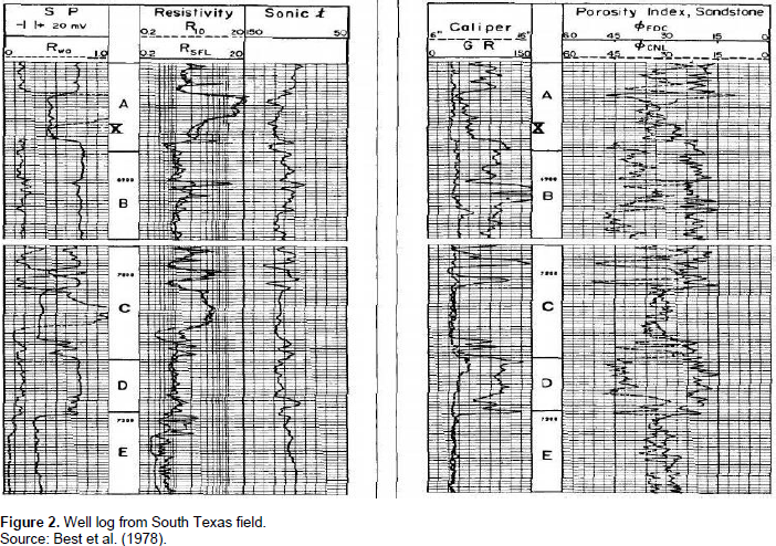
The average reservoir temperature for the South Texas field was reported to be 150°
F, and the Neutron log reported sandstone lithology while the SP and GR logs indicated different proportions of shales. The South Texas section of interest has been divided into four intervals. Interval A contains shaly hydrocarbon-bearing sand, which has a gas cap indicated by separation of the neutron and density porosities. Interval B is mostly shale with some thin sands and can be used to select shale parameters. Interval C contains hydrocarbon-bearing sands while Interval D contains reasonably clean water sand, as presented by Best et al
. (1978) in Figure 2. To help in identification of shale distribution mode and to use it for selection of the suitable model for calculating water saturations in the South Texas field, readings are obtained from sections of interest of the logs from a well in the South Texas field (Best et al., 1978), as shown in Figure 2. Shaly sand sections are corresponding to depths 6,880 ft to 6,940 ft in the well. For this shaly sand section, the corresponding parameters are read at 10 different depths and used to calculate water saturation using different shaly sand models.
The parameters and well logging readings are used in the comparison of water saturation models and listed below in Table 1. The Gamma ray values are used in shale volume (Vsh) calculations because it indicates lower values for shale volume than those from the SP log, Table 1. The total porosity (φ) is calculated as a mathematical average of neutron and density porosities (φN and φD), respectively. The modified resistivity factor (F*) for shaly formation is plotted versus porosity. This is known as a modified Picket plot of log (F*) versus log (φ). This plot is used to obtain values for modified tortuosity (a*) and modified exponent (m*) for shaly formation of this field. The value of a* is obtained as the value of φ at the intersection of the x-y axis, and m* is obtained as negative slope of the line in the log-log plot.

The parameter q involved in the dispersed shale model is called the sonic response and is calculated using values of sonic and density porosity as; {q = (φs+ φD) / φs }. The data listed in Table 1 is used to compute water saturation using five shaly sand water saturation models and the results attained are presented in Table 2. The calculated values of shale volume and water saturation are graphically presented in Figure 3. Figure 3 compares the shale volume and water saturation (Sw) values using five different models as a function of depth in the shaly sand zones of the South Texas field.
For the South Texas field, as shown in Figure 3, the dispersed shale model overestimates values of water saturation, while the laminated shale model provides underestimated values, relatively to the total shale model, which is indifferent to shale distribution.

Although there is a big difference in the values of the dispersed shale model and the laminated shale model, however, they followed a similar responsiveness and pattern to the total shale model and shale volume (Vsh) curve. This may reveal that both laminated and dispersed distributions exist homogenously in the South Texas field. This conclusion is based on the fact that the average of the laminated and dispersed shale models resulted averagely to the curves of the remaining shaly sand water saturation models, which takes all shale distribution modes into account. The results of the total shale model, Simandoux equation, and Indonesian model show very similar values overall with insignificant variance in the results (Figure 3). This similarity between these three models may indicate proper estimation of the values of tortuosity factor (a), cementation factor (m), and saturation exponent (n). It also indicates the applicability of all three models for the South Texas field.
Based on the results attained from comparing different water saturation models, it is imperative to identify the shale distribution in the formation to select the appropriate model for accurate calculations. For identification of shale distribution, the technique of plotting the porosity derived from neutron and density logs is applied (Institute of Petroleum Engineering (IPE), 2014). The actual data from the South Texas well is plotted on this triangle and location of plotted data indicates the distribution mode of shale. This crossplot of neutron (φN) - density (φD) porosity is presented in Figure 4.Figure 4 has been used in the oil industry to identify the shale distribution mode. It is mainly a plot of density porosity versus neutron porosity on y and x axes, respectively. Distribution of data points in Figure 4 indicates that the South Texas field exhibit both laminated and structural shale distribution homogenously across the reservoir. This means using another saturation model rather than laminated one provides erroneous results.

North Sea field
Actual well log from the North Sea field is presented by Institute of Petroleum Engineering (IPE) (2014), as shown in Figure 5. The shaly sand sections of interest correspond to depths from 11,870 to 11,880 ft in the North Sea field. For shaly sand sections, the corresponding parameters are read at 10 different depths, and used to calculate water saturation using five different shaly sand models. Readings of different well logs plus constants and parameters for the shaly sand zones are listed versus depth in Table 3. Five different shaly sand models are used to calculate the water saturation and the obtained results are listed in Table 4 for the North Sea field and graphically presented in Figure 6. Figure 6 compares the attained values of water saturation computed using different models versus depth in the shaly sand zones of interest of the North Sea field.


For the North Sea field, as shown in Figure 6, the Indonesian shale model yielded the lowest values of water saturation (Sw) while the total shale model provided exceptionally the highest values. This figure also presented the water saturation calculated using Archie’s equation, which lies in the middle between these two extreme cases. As for the same graph (Figure 6), the total shale model also gave high estimates of Sw, while the Simandoux equation showed slighter lower values, and the Indonesian model shows very low values of Sw. This highly estimated value using the total shale model is mostly attributed to the generous assumption in the total shale model that m = n = 2 for all reservoirs. This shows that proper estimation of the values of m and n have a real impact on the estimated water saturation values. This big variance between the total shale model, Simandoux equation, and Indonesian model, may indicate poor attribution for the estimated values of tortuosity factor (a), cementation factor (m), and saturation exponent (n). This may be caused due to the poor estimate of water resistivity (Rw).
The calculated water saturation (Sw) using the dispersed shale model between depths 11,873 and 11,876 ft in Figure 6 shows an extreme boost in values of Sw that occurred with the sudden increase in shale volume (Vsh) which could be described as an abnormality. This may be attributed to improper selection of the dispersed shale model for this particular field. On the other hand, the laminated shale model followed an almost similar responsiveness and pattern to the remaining water saturation models in shaly sand, particularly the total shale model. It is essential to properly describe shale distribution and verify the quality and accuracy of input parameters in order to select the correct shaly sand model for calculation of water saturation. The neutron-density porosity crossplot of the North Sea field is presented in Figure 7 and used to identify the shale distribution in the North Sea field. The plot of Figure 7 indicates that North Sea field mostly inhibits dispersed shale distribution.

Variation of the tortuosity coefficient (a), cementation exponent (m) and saturation exponent (n) has been studied. A sensitivity analysis is carried out to study the effect of applying different values of a and m on values of water saturation using the laminated shale model. The Indonesian model is used to study the effect of saturation exponent (n) because it is the only model involving that exponent (n). Figure 8 graphically presents the calculated values of water saturation using different values of tortuosity coefficient (a) versus depth for all-selected models. A conclusion can be drawn that the increase of tortuosity coefficient (a) results in an increase in calculated values of water saturation for all shaly sand models.

The effect of variable values of the cementation exponent (m) on water saturation versus depth is achieved and the results are plotted in Figure 9 which reveals that the increase of m values increases the computed values of water saturation in shaly sandstone reservoirs. The Indonesian water saturation model is used to perform a sensitivity analysis about the effect of applying different values of the saturation exponent (n) on the saturation values calculated. The results are presented in Figure 10. The increase of cementation exponent (m) causes an increase in water saturation calculated using the Indonesian model. The increase of saturation exponent (n) leads to an increase in water saturation calculated (Figure 10). A simple comparison of the effects of n, m, and n on water saturation (Figures 8, 9 and 10), respectively, indicates that the m exponent has the highest impact while the tortuosity factor (a) has the lowest one.
Comparison and evaluation of different shaly sand models is achieved and sensitivity analysis of the tortuosity factor, cementation and saturation exponents is carried out in this study. The attained conclusions are summarized as follows:
(1) Identification of the shale distribution in the reservoir is crucial for selecting the appropriate model for calculating the water saturation in shaly sand reservoirs.
(2) The increase of shale volume decreases the calculated values of water saturation using all shaly sand models.
(3) Different shaly sand water saturation models inhibit a drastic variance in estimated water saturation which may exceed 60% in difference.
(4) The laminated shale model provides the lowest value of water saturation while the total shale model produces the highest one.
(5) Application of Simandoux, Indonesian and total shale models provides comparable results of water saturation in shaly sand reservoirs.
(6) Overestimation of the tortuosity factor (a) and cementation exponent (m) causes an overestimation of water saturation calculated using all models.
(7) Overestimation of the saturation exponent (n) results in an underestimation of water saturation calculated using all models.
(8) Total shale model showed the highest degree of responsiveness to variance in shale volume of all shaly sand water saturation models.
The authors have not declared any conflict of interests.