Full Length Research Paper

ABSTRACT
Earth's magnetosphere is a magnetic shield that protects the Earth from the energetic emissions of the high-speed Solar Wind (HSSW). We perform a statistical analysis of the response of Earth's magnetosphere inner part under the impact of HSSW over 40 years of data encompassing solar cycles 20-23. With misidentified events or events interacting with interplanetary coronal mass ejections (ICMEs) removed, only 23552 events were identified. The results we obtained show that more than 85% of the events recorded from 1964 to 2009 are generated by coronal holes (CHs). Almost all observations were confined between 250-800 km/s and show a unimodal distribution per solar cycle: (1) 93% of the solar wind (SW) velocities are on the order of 567.77 ± 2.46 km/s for solar cycle 20, (2) 81% of the SW velocities are worth 524.30 ± 2.69 km/s for cycle 21, (3) 92% of the SW velocities progress to 565.15 ± 2.72 km/s for cycle 22, and (4) 75% of the SW velocities show a value on the order of 530.38 ± 2.22 km/s for cycle 23. Furthermore, our analysis shows a lower electron density at the beginning of the cycle (48%) than at the end of the solar cycle (52%). Thus HSSWs are more frequent at the end of solar cycles, while the magnetospheric electric field (EM) instead shows dominant features during the upward phase of odd cycles and the downward phase of even cycles. Therefore, the stability of the inner magnetosphere is more significant during the decline of solar cycles.
Key words: High-speed solar winds, magnetospheric electric field, interplanetary coronal mass ejections.
INTRODUCTION
Space weather refers to solar phenomena and environments that can affect the operation and reliability of space and ground-based systems and services, or even threaten human health (Schwenn, 2006; Belisheva et al., 2019; Abdullrahman and Marwa, 2020; Hapgood et al., 2021). All of these disturbances have socio-economic consequences whose cost can only be properly assessed with an accurate knowledge of climate variability. The phenomena representing one of the key factors of perturbations of the solar environment are the coronal holes (CHs). It is generally accepted that HSSWs originates from CHs and associated corotating interaction regions (Krieger et al., 1973; Sheeley et al., 1976; McComas et al., 1998; Richardson et al., 2000; McGregor et al., 2011b; Zerbo et al., 2012). Structure of the solar wind (SW) evolves as it flows outward through the heliosphere away from Sun. Through corotation of polar CHs associated with the "open" magnetic flow or through solar flare activity, HSSWs are created (Poletto, 2013; Owens et al., 2017). Ejected from the Sun and traveling through interplanetary space, HSSWs carry highly energetic particles; resulting in an increase in the mean interplanetary magnetic field (IMF). SW interacts with the CMI Bi and generates a VSW × Bi electric field that crosses the magnetosphere. The latter interacts with the Earth's magnetic field and generates a force that controls the convective motion of the magnetospheric plasma. EM field thus plays a very important role on the dynamics of the Earth's magnetosphere. Indeed, according to Baumjohann et al. (1985), part of the EM field is driven by the ionospheric dynamo. Matsui (2003) showed that the magnetospheric source contributes at least 30% of the electric field, while the ionospheric dynamo contributes at least 25%. In addition, numerous quiet-time studies of the characteristics of environmental changes in the magnetospheric plasma due to HSSW have been performed (Harvey and Sheeley, 1978; Sheeley and Harvey, 1981; Verbanac et al., 2011a, b). However, the overall variation in the energy potential of HSSWs in magnetically perturbed periods (Aa ≥ 20 nT) remains unknown, and the response of this solar-phase variability on EM field for cycles 20 to 23 is not yet clarified.
To quantify the study of solar winds, a consistent definition of what is meant by HSSW is needed. Indeed, many definitions have been proposed for HSSW over time. According to Bame et al. (1976) and Gosling et al. (1976), a HSSW is an observed variation in SW velocity, with an increase in velocity of at least 150 km/s within a five-day interval. Broussard et al. (1978) described it as a flow with a velocity greater than 500 km/s averaged over one day. In addition, Lindblad and Lundstedt (1981) defined it as a flow defined over a period during which the difference in velocity between the lowest value on 03 h and the highest on 03 h of the following day, is greater than 100 km/s and it lasts at least two days. Later, according to Mavromichalaki et al. (1988), and Mavromichalaki and Vassilaki (1998), HSSW is a flow defined over a period in which the difference between highest and average velocity of the plasma immediately preceding and following the flow, is greater than 100 km/s over an interval of at least two days. And finally, Intriligator (1973, 1977), Richardson and Hilary (2012), Zerbo et al. (2012), Villarreal et al. (2014) and Despirak et al. (2019) described it as a rapid increase in SW flux with a peak velocity greater than or equal to 450 km/s on average. The latter definition would be used in the present study because, we believe, it mostly covers the limit imposed according to other authors. A typical example of the velocity variation of the whole solar wind for the year 1994 is shown in Figure 1.
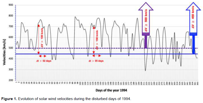
Year 1994 is chosen because of the frequent occurrence of intense activity (Tanskanen et al., 2005; Reeves et al., 2011). In this Figure 1, SW velocities beyond the horizontal plot (blue plot) are greater than or equal to 450 km/s day. We note that more than 80% of the SW velocities for year 1994 coincide with the definition of a HSSW given earlier. This article discusses this topic, in particular the effect of long-term HSSW variability on the EM field. In this manuscript, we will examine the geoeffectiveness of the Earth's magnetosphere during daytime magnetic reconnection in the face of intense HSSW fluctuations. The main reason for studying long-term HSSWs is that they are a potential hazard to the Earth and to space systems.
Many studies have shown that the solar flux is strongly dependent on the long-term solar cycle and activity (Joshi et al., 2011; Zerbo et al., 2013; Elena et al., 2013; Shinichi, 2017). Indeed, according to Snyder et al. (1963) and Svalgaard (1977), geomagnetic activity depends on the parameters of the SW, in particular its velocity. Thus, several authors have grouped geomagnetic activity into four standard classes (Ouattara et al., 2009; Du, 2011) based on the former classification made by other authors (Legrand and Simon, 1981, 1989; Simon and Legrand, 1989; Richardson et al., 2000, 2002). Later, Ouattara et al. (2009) and Zerbo et al. (2012) reported a new extension of the standard classification by scrutinizing with new solar wind conditions, the global classification established by Legrand and Simon (1981, 1989). This new extension allowed Zerbo et al. (2012) to clearly identify about 80% of the geomagnetic activity today, compared to 60% identified by Legrand and Simon (1981, 1989). In this study, the new extension of Zerbo et al. (2012) will be used and we will restrict ourselves to magnetically disturbed periods, which are characterized by geomagnetic indices Aa ≥ 20 nT (Ouattara et al., 2009; Zerbo et al., 2012).
DATA AND METHODOLOGY
Data set
In this paper, various spatial datasets available in the public domain were used. Hourly observations of SW parameters compiled by the scientific community and available via the OMNIWeb link «http://omniweb.gsfc.nasa.gov/form/dx1.html» are used to obtain information relating to the frozen electric field (Ey) in SWs and the velocity of these SWs. To examine the geomagnetic indices (Aa) evaluated by 03 h resolution, data available on «http://isgi.unistra.fr/» were used to obtain relative information on magnetically disturbed days from 1964-2009 period. It is important to note that no reliable information on the structure of the Ey field in the SW was available for the first half of the year 1964. For this study, based on the Wolf numbers (Rz) available at «http://sidc.oma.be/sunspot-data/», the exact start/end periods of the ascending and descending phases of the four solar cycles 20-23 studied via the link «http://users.telenet.be/j.janssens/Engzonnecyclus.html#Overzicht» have been summarized in Table 1.

Approach
We analyze continuous data over the range 1964-2009 only for disturbed periods, which are identified by geomagnetic indices Aa ≥ 20 nT. According to Legrand and Simon (1989), Richardson and Hilary (2012), Zerbo et al. (2012) and Despirak et al. (2018), these periods represent the manifestation class of HSSW. First, we remove all unreliable information from the solar flux velocities Vsw and the hourly Ey field into this flux over the long 45-year period. Note that the Ey field is in most cases, the dominant factor that determines the structures of the high latitude EM field as well as the magnetospheric convection processes associated with it. Thus, component of the total electric field related to the corotation of the Earth, will be neglected in this article. After filtering, Ey field [mV/m] is used to determine EM field [mV/m] using the relation of Wu et al. (1981), later validated by Revah and Bauer (1982):

Secondly, annual average values of the EM and Vsw parameters are estimated. These averages remove the periodicities associated with shorter time scales. The use of average values in this study compensates for the effects of day-to-day variability of the Sun's activity in the proxies used. Since, the objective in this paper is to study the global variations of HSSW and their impact on the EM field during perturbed periods, it would be reasonable to use average parameters for an overall view.
Furthermore, to check our data for a significant difference per solar cycle in the velocity distribution of HSSW and EM field, recourse was made to the Kolmogorov - Smirnov (KS) test «http://www.physics.csbsju.edu/stats/KS-test.html». KS test statistic measures the largest Dks distance between empirical distribution function of the processed data and hypothesized distribution (Stephens, 1992). It is important to note that KS test is a non-parametric goodness-of-fit test that is widely used in statistical studies. KS test gives a 95% confidence interval for true means against a fixed 5% risk of error (Wilks, 2011; Jesper, 2014). Based on the number of data points, the statistical value Dks varies, which is the maximum difference between the cumulative distributions of two selected data sets. The critical values  (Equation 2) with n, the number of events, indicate whether the selected data, differ significantly (Gabriel, 2014).
If is greater than Dks, the null hypothesis of no difference between the data sets is rejected (Lilliefors, 1967; Crutcher, 1975; Ruppert, 2004; Steinskog et al., 2007; Vlcek and Huth, 2009; Wilks, 2011).
RESULTS AND DISCUSSION
Distribution of high-speed solar winds
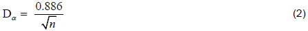
Figure 2 shows the statistical distribution of HSSWs during magnetically perturbed periods for all solar cycles 20-23. Panels (a), (b), (c), and (d) represent the statistical distribution of all solar winds for solar cycles 20, 21, 22, and 23, respectively. The analysis of all these panels shows that more than 99% of the solar wind velocities are in the range 250-800 km/s, which is identified by several authors (McGregor et al., 2011a; Villarreal et al., 2014; Rotter et al., 2015). However, according to Figure 2, not all HSSWs have a peak velocity ≥ 450 km/s, as pointed out by several publications (Intriligator, 1973, 1977; Richardson and Hilary, 2012; Zerbo et al., 2012; Villarreal et al., 2014; Despirak et al., 2018). Indeed, examination of panels (a), (b), (c), and (d) in Figure 2 shows that at least 93, 81, 92 and 75% of the SW velocities blowing on disturbed days, respectively, are greater than or equal to 450 km/s. We note that the even cycles (20 and 22) have a high rate of occurrence of HSSW compared to the odd cycles (21 and 23). From this analysis, it is therefore clear that high-speed solar flux is the main contributor at about 85% to the SW solar averages during magnetically disturbed periods. This contribution is in very good agreement with the work of Legrand and Simon (1989), Lindblad (1990), Richardson et al. (2000), Zerbo et al. (2012) and Bharati et al. (2019) in which, SW velocity limit is set to characterize the period of magnetically disturbed days.
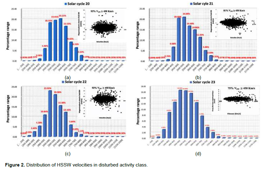
Our statistical study shows us to what extent, distributions of HSSWs during perturbed periods are not all similar for the four solar cycles or at least for the interval considered, whatever the solar flux variation (Zerbo et al., 2012; Bharati et al., 2019). Despite the smaller changes in HSSWs from one solar cycle to the next in magnetically perturbed periods; overall, their average variations during the rise and fall of solar phases follow closely. Indeed, according to Figure 3(b), the average velocities of HSSWs corresponding to the ascending and descending phases of the four solar cycles studied are of the order of 48 and 52% respectively of the total flux. In fact, Figure 3(a) shows dominant features during the descent phase: average velocities increase, reaching their highest values. These results are in very good agreement with the work of several authors (Bame et al., 1976; Gazis, 1996; Richardson et al., 2002; Luhmann et al., 2009; Jacob et al., 2020). The peak velocities of solar cycles 20 to 23 obtained during the ascending phases are respectively 541.90, 546.20, 546.67 and 516.95 km/s against 598.04, 557.96, 599.78 and 576.48 km/s for the descending phase. These peaks would be related to several coronal holes (CHs) which are known to generate high-speed solar flows (Lindblad, 1990; Echer et al., 2004). The dominant characteristics of the velocities at the end of the solar cycle suggest that the mass transport towards the Earth intensifies in this period. Consequently, the internal magnetosphere becomes unstable at the end of the solar cycle than at the beginning during magnetically disturbed periods. On the one hand, this result is in good agreement with the simulations of stable magnetospheric convection made by Pulkkinen et al. (2007); and on the other hand, by many other authors (Phillips et al., 1995; Ebert et al., 2009). In addition, during the descending phases of solar cycles, HSSWs velocities are so great that "bow shocks" could form whenever they are forced to travel around the planets of the solar system. Such bow shocks will also form around airplanes, rockets, or the space shuttle when these vehicles travel faster than the speed of sound through the atmosphere.

It is important to note that during the ascending phase, corotating flows have average speeds (Vsw) between 450 and 500 km/s, while they are above 500 km/s during the descending phase. Since the strength of a solar flux is generally characterized by stable magnetospheric convection events, we estimate that there are a significant number of magnetic storms at the end of the solar cycle than at the beginning. Such events at the end of the solar cycle, suggested that the Earth's environment, and perhaps even the Sun, are sources of disruptions and failures in new technologies such as wireless communications and power systems on a local and geographical scale. These notable features are corroborated by the work of Ouattara (2015), Kabore? and Ouattara (2018), and Despirak et al. (2018) where the storms were named "expanded substorms" for Vsw > 500 km/s and "polar substorms" for Vsw < 500 km/s. The increase in HSSW velocities at the end of the solar cycle noted in this paper, makes the outer layers of the plasmasphere convectively unstable and consequently, able to generate many irregularities in the plasmapause region. This aspect of trends is justified by the fact that electron fluxes are seasonally dependent. Indeed, Yeeram (2020) proved that electron fluxes are relatively low during the ascending phases of solar cycles and high during the descending phase. Our results are consistent with this argument when the corresponding periods are compared.
Magnetospheric response in perturbed periods
For a better understanding of the impact of HSSWs on the EM field during the ascending and descending phases of solar cycles, we have plotted histograms of EM field for the class of magnetically disturbed periods in Figure 4a. It appears that even cycles (20 and 22) exhibit dominant characteristics of the EM field during the descending phase. On the other hand, odd solar cycles (21 and 23) show rather a high proportion of the EM field during the ascending solar phase. The notable features observed during the even cycles may be due to the fluctuations and large amplitudes recorded in these cycles.
In order to conclude whether or not the two means of the magnetospheric electric field come from the same population during the ascending and descending solar phases, we performed a T-test. The significance levels of the EM field, recorded in Table 2, are all satisfactory (p < 0.05), so we prove the satisfaction of our results. The results of the T-test confirm once again that the averages of the EM field come from the same type of sample analyzed.
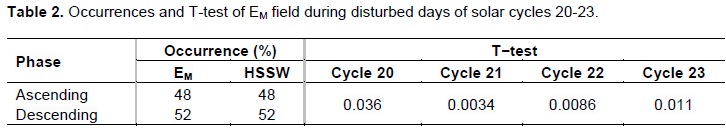
Examination of columns 2 and 3 of Table 2 tells us that HSSW and EM field constantly evolve in phase for all the solar cycles studied. This is justified by the similarity of the distributions observed in Figures 3b and 4b. However, special attention is given to the rather large occurrence of the EM field observed during the downward phase of solar cycle 22 (Figure 4a). Indeed, solar cycle 22 reveals the existence of typical abrupt variations of the EM field and of large amplitudes of HSSWs. This contribution is corroborated by the work of Inza et al. (2022).
In addition, the study of solar wind particles, and particularly HSSW, are very complex random phenomena. Thus, the distribution of solar flux velocities is made more useful through statistical methods. For this reason, the probabilities of HSSW velocities can be estimated using probability distributions. Since we have only considered magnetically perturbed days in this paper, we do not expect much change in HSSW averages. An accurate determination of the probability distribution of the average HSSW velocities is very important for assessing the solar wind energy potential of a given solar phase/cycle. Instead of computing a full distribution over the features to approximate an underlying process, we will restrict ourselves to the distribution of the properties of these features over a finite number of points for 1964-2009 period. Thus, analysis of the long data set of HSSW particles by the KS test gives very satisfactory results. Indeed, the Dks statistical values are all greater than or equal to the critical values for both solar quantities. Particular attention is paid to the critical values, which are all below the fixed risk of error (5%). These arguments show the consistency of the selected data sets, and therefore, indicate that the velocity distributions of HSSW and EM field are similar over 03-h cadences. However, for even solar cycles, the statistical values of HSSW are higher than those of EM field, while the opposite is found for odd cycles. The differences between even and odd cycles have in the Sun, a very random character. According to Durney (2000) and Takalo (2021), these differences are related to the amplitudes and/or Gnevyshev gaps (GG) between the ascending and descending phases of the solar cycles. One could estimate that the Dks statistical values are related to the nature of the solar cycles and the size of the samples. The results of KS test are given in Table 3.
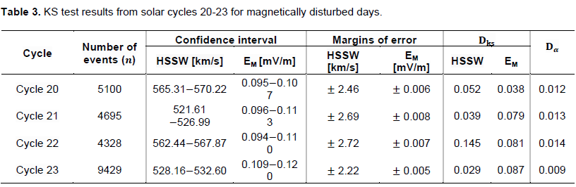
Moreover, when it comes to determining the practical significance of a set of processed data, confidence intervals are generally more useful than tests (Nick et al., 2003; Jean-Baptist et al., 2009; Ranstam, 2012). In the case of comparing two population means of solar winds, it is important to construct a confidence interval and conclude that there is an effect of practical significance only if all differences in that interval are small enough. According to Ruppert (2004), if the difference in the confidence interval is high, then the information is less accurate. Therefore, a lower confidence interval is more likely to return the correct value. In this manuscript, the difference in confidence intervals for HSSWs, although small, is greater (2.22 to 2.72 km/s) than for EM fields (0.005 to 0.008 mV/m) as can be observed in columns 5 and 6 of Table 3. We could therefore conclude with a 95% confidence level that there is no significant difference for the processed data set. The difference in the margins of error between our two populations is probably due to the size of the samples analyzed. Indeed, the EM field values are relatively small compared to the HSSW values. It is therefore clear that the confidence intervals are strongly influenced by the sample size. This analysis is corroborated by the results of Tukur (2008).
CONCLUSION
Various examples of perturbed events and their effect on the inner magnetosphere discussed here, with particular emphasis on the changes associated with the progression of solar cycles 20-23 to the averages of the geomagnetic indices (Aa), have been realized for the period extending from 1964 to 2009. Stable currents of large amplitudes (from peak to trough greater than or equal to 450 km/s) were most often observed during the years of descending phases: about 570.22 km/s in 1974 (cycle 20), about 526.99 km/s in 1986 (cycle 21), about 567.87 km/s in 1994 (cycle 22), and about 532.60 km/s in 2003 (cycle 23). This aspect of solar flux velocity variation is reflected in the 5-95% range of velocity values listed in column 3 of Table 3. The results by means of the statistical tests (T-test, KS test and 95% confidence interval) which we arrived at indicate a better distribution of the selected data. However, these results are more significant for the EM field than for the HSSW. Moreover, the statistical analysis of the energetic particles in the solar flux confirms that about 85% of the SW represents the main contributor to HSSWs during magnetically disturbed periods. The presence of dominant HSSW features at the end of the solar cycle significantly affects the stability of the day-side inner magnetosphere. Across the 20-23 solar cycles, HSSW and EM field recorded a small contribution (48%) during the ascending phase compared to 52% of solar averages during the descending phase of solar cycles. These results support the hypothesis that HSSW and EM quantities controlling the state of the inner magnetosphere, evolve in phase during the ascending and descending phases of solar cycles. Despite the obvious importance of the EM field on a large scale, their observation is very difficult because of its very complex spatial and temporal structure and its low variability in space and time. Of the solar cycles studied, even cycles (20 and 22) showed dominant EM field characteristics during the descending phase while the odd cycles (21 and 23) rather showed a high proportion of EM field during their ascending phases. In addition to the threat to spacecraft systems posed by characteristic dominants, the radiative environment of space also poses risks to the health and safety of astronauts. Appropriate measures must therefore be pursued to minimize astronaut exposure to HSSW particle emissions during geomagnetic storms and solar energy.
CONFLICT OF INTERESTS
The authors have not declared any conflict of interests.
ACKNOWLEDGMENTS
The authors are very grateful to the space data centers OMNIWeb and CDPP for the quality of the solar wind structure data and ISGI for the geomagnetic index data.
REFERENCES
|
Abdullrahman HM, Marwa AM (2020). The Effects of Solar Activity and Geomagnetic Disturbance on Human Health. Open Access Journal of Biomedical Science 2(5). |
|
|
Bame SJ, Asbridge JR, Feldman WC, Gosling JT (1976). Solar cycle evolution of high-speed solar wind streams, Astrophysical Journal 207(3):977-980 |
|
|
Baumjohann W, Haerendel G, Melzner F (1985). Magnetospheric convection observed between 0600 and 2100 LT: Variations with Kp. Journal of Geophysical Research 90(A1):393-398. |
|
|
Belisheva NK, Kanao M, Kakinami Y, Toyokuni G (2019). The Effect of Space Weather on Human Body at the Spitsbergen Archipelago. Arctic Studies - A Proxy for Climate Change, IntechOpen. |
|
|
Bharati K, Amar K, Durbha SR, Gurbax SL (2019). Diminishing activity of recent solar cycles (22-24) and their impact on geospace. Journal of Space Weather and Space Climate 9(A1). |
|
|
Broussard RM, Sheeley NR, Tousey R, Underwood JH (1978). A survey of coronal holes and their solar wind associations throughout sunspot cycle 20. Solar Physics 56(1):161-183. |
|
|
Crutcher HL (1975). A note on the possible misuse of the Kolmogorov- Smirnov test. Journal of Applied Meteorology 14:1600-1603. |
|
|
Despirak IV, Lubchich AA., Kleimenova NG (2018). High-latitude substorm dependence on space weather conditions in solar cycle 23 and 24 (SC23 and SC24). Journal of Atmospheric and Solar-Terrestrial Physics 177:54-62. |
|
|
Despiraka IV, Lyubchicha AA, Kleimenovab NG (2019). Solar Wind Streams of Different Types and High-Latitude Substorms. Geomagnetism and Aeronomiy 59(1):1-6. |
|
|
Du ZL (2011). The correlation between solar and geomagnetic activity - Part 1: Two-term decomposition of geomagnetic activity. Annales Geophysicae 29(8):1331-1340. |
|
|
Durney BR (2000). On the differences between odd and even solar cycles. Solar Physics 196(2):421-426. |
|
|
Ebert RW, McComas DJ, Elliott HA, Forsyth RJ, Gosling JT (2009). Bulk properties of the slow and fast solar wind and interplanetary coronal mass ejections measured by Ulysses: Three polar orbits of observations. Journal of Geophysical Research: Space Physics 114(A1) |
|
|
Echer E, Gonzalez W, Gonzalez AL, Prestes A, Vieira LE, Dal LA, Guarnieri FL, Schuch NJ (2004). Long-term correlation between solar and geomagnetic activity. Journal of Atmospheric and Solar-Terrestrial Physics 66(12):1019-1025. |
|
|
Elena S, Yolanda C, Consuelo C, Venera D, Pavel H, Petko N, Peter S, Josef B, Dimitar D, Crisan D, Walter DG, Georgeta M, Dimitar T, Fridich V (2013). Geomagnetic response to solar and interplanetary disturbances. Journal of Space Weather and Space Climate 3(A26). |
|
|
Gabriel CB (2014). Revisiting the critical values of the Lilliefors test: towards the correct agrometeorological use of the Kolmogorov- Smirnov framework, Bragantia, Campinas 73(2):192-202. |
|
|
Gazis PR (1996). Solar cycle variation in the heliosphere. Reviews of Geophysics 34(3):379-402. |
|
|
Gosling JT, Asbridge JR, Bame SJ, Feldman WC (1976). Solar wind speed variations: 1962-1974. Journal of Geophysical Research, 81(28):5061-5070. |
|
|
Hapgood M, Angling MJ, Attrill G, Bisi M, Cannon PS, Dyer C, Eastwood P, Elvidge S, Gibbs M, Harrison RA, Hord C, Horne RB, Jackson DR, Jones B, Machin S, Mitchell CN, Preston J, Rees J, Rogers NC, Routledge G, Ryden K, Tanner R, Thomson AWP, Wild JA, Willis M (2021). Development of Space Weather Reasonable Worst-Case Scenarios for the UK National Risk Assessment. Space Weather 19(4). |
|
|
Harvey JW, Sheeley NR (1978). Coronal holes, solar wind streams, and geomagnetic activity during the new sunspot cycle. Solar Physics, 59(1):159−173. |
|
|
Intriligator D (1973). Report UAG-27, WDCA Solar Terr. Phys., Boulder. |
|
|
Intriligator D (1977). In M. Shea et al. (eds.), Study of Travelling Interplanetary Phenomena, D. Reidel Pub!. Co., Dordrecht, Holland 195 p. |
|
|
Inza G, Christian Z, Salfo K, Frédéric O (2022). Variability of the magnetospheric electric field due to high-speed solar wind convection from 1964 to 2009. African Journal of Environmental Science and Technology 16(1):1-9. |
|
|
Jacob O, Yu L, Amobichukwu CA, Mingyu Z (2020). Responses and Periodic Variations of Cosmic Ray Intensity and Solar Wind Speed to Sunspot Numbers, Advances in Astronomy pp. 1-10. |
|
|
Jean-Baptist du P, Gerhard H, Bernd R, Maria B (2009). Confidence Interval or P-Value? Review article 106(19):335-339. |
|
|
Jesper WS (2014). Null hypothesis significance tests. A mix-up of two different theories: the basis for widespread confusion and numerous misinterpretations. Scientometrics 102(1):411-432. |
|
|
Joshi NC, Bankoti NS, Pande S, Pande B, Pandey K (2011). Relationship between interplanetary field/plasma parameters with geomagnetic indices and their behavior during intense geomagnetic storms. New Astronomy 16(6):366-385. |
|
|
Kabore? S, Ouattara F (2018). Magnetosphere convection electric field (MCEF) time variation from 1964 to 2009: Investigation on the signatures of the geoeffectiveness coronal mass ejections. International Journal of Physical Sciences 13(20):273-281. |
|
|
Krieger AS, Timothy AF, Roelof EC (1973). A coronal hole and its identification as the source of a high velocity solar wind stream. Solar Physics, 29(2):505-525. |
|
|
Legrand JP, Simon PA (1981). Ten cycles of solar and geomagnetic activity. Solar Physics 70(1):173-195. |
|
|
Legrand JP, Simon PA (1989). Solar cycle and geomagnetic activity: a review for geophysicists. Part I. The contributions to geomagnetic activity of shock waves and of the solar wind. Annales Geophysicae 7(6):565-578. |
|
|
Lilliefors HW (1967). On the Kolmogorov-Smirnov test for normality with mean and variance unknown. Journal of the American Statistical Association 62(318):399-402. |
|
|
Lindblad BA (1990). Coronal sources of high-speed plasma streams in the solar wind during the declining phase of solar cycle 20. Astrophysics and Space Science 170(1-2):55-61. |
|
|
Lindblad BA, Lundstedt H (1981). A Catalogue of High-Speed Plasma Streams in the Solar Wind. Physics of Solar Variations, 197−206. |
|
|
Luhmann JG, Lee CO, Li Y, Arge CN, Galvin AB, Simunac K, Petrie G (2009). Solar wind sources in the late declining phase of cycle 23: Effects of the weak. Solar Physics 256(1):285-305. |
|
|
Matsui H, Quinn JM, Torbert RB, Jordanova VK, Baumjohann W, Puhl-Quinn PA, Paschmann G (2003). Electric field measurements in the inner magnetosphere by Cluster EDI, Journal of Geophysical Research 108(A9). |
|
|
Mavromichalaki H, Vassilaki A (1998). Fast plasma streams recorded near the earth during 1985-1996. Solar Physics, 183(1):181−200. |
|
|
Mavromichalaki H, Vassilaki A, Marmatsouri E (1988). A catalogue of high-speed solar-wind streams: Further evidence of their relationship to Ap-index. Solar Physics 115(2):345-365. |
|
|
McComas DJ, Bame SJ, Barraclough BL, Feldman WC, Funsten HO, Gosling JT, Riley P, Skoug R, Balogh A, Forsyth R, Goldstein BE, Neugebauer M (1998). Ulysses' return to the slow solar wind. Geophysical Research Letters 25(1):1-4. |
|
|
McGregor SL, Hughes WJ, Arge CN, Odstrcil D, Schwadron NA (2011b). The radial evolution of solar wind speeds. Journal of Geophysical Research 116(A3). |
|
|
McGregor SL, Hughes WJ, Arge CN, Owens MJ, Odstrcil D (2011a). The distribution of solar wind speeds during solar minimum: Calibration for numerical solar wind modeling constraints on the source of the slow solar wind, Journal of Geophysical Research 116(A3). |
|
|
Nick C, Graeme DR (2003). Confidence intervals are a more useful complement to nonsignificant tests than are power calculations, Behavioral Ecology 14(3):446-447. |
|
|
Ouattara F, Amory-Mazaudier C (2009). Solar-geomagnetic activity and Aa indices toward a standard classification. Journal of Atmospheric and Solar-Terrestrial Physics 71(17-18):1736-1748. |
|
|
Ouattara F, Nour AM, Franc?ois Z (2015). A Comparative Study of Seasonal and Quiettime fof2 Diurnal Variation at Dakar and Ouagadougou Stations during Solar Minimum and Maximum for Solar Cycles 21-22. European Scientific Journal 11(24). |
|
|
Owens MJ, Lockwood M, Riley P (2017). Global solar wind variations over the last four centuries. Scientific Reports 7(1). |
|
|
Phillips JL, Bame SJ, Barnes A, Barraclough BL, Feldman WC, Goldstein BE, Gosling JT, Hoogeveen GW, McComas DJ, Neugebauer M, Suess ST (1995). Ulysses solar wind plasma observations from pole to pole. Geophysical Research Letters 22(23):3301-3304. |
|
|
Poletto G (2013). Sources of solar wind over the solar activity cycle, Journal of Advanced Research 4(3):215-220. |
|
|
Pulkkinen TI, Goodrich CC, Lyon JG (2007). Solar wind electric field driving of magnetospheric activity: Is it velocity or magnetic field?Geophysical Research Letters 34(21):L21101. |
|
|
Ranstam J (2012). Why the P-value culture is bad and confidence intervals a better alternative, OsteoArthritis Society International 20(8):805-808. |
|
|
Reeves GD, Morley SK, Friedel RHW, Henderson MG, Cayton TE, Cunningham G, Blake B, Christensen AR, Thomsen D (2011). On the relationship between relativistic electron flux and solar wind velocity: Paulikas and Blake revisited. Journal of Geophysical Research: Space Physics 116(A2). |
|
|
Revah I, Bauer P (1982). Rapport d'activite? du Centre de Recherches en Physique de l'environnement Terrestre et Plane?taire, Note technique CRPE/115, 38-40 Rue du Ge?ne?ral Leclerc 92131 Issy-Les Moulineaux. |
|
|
Richardson IG, Cane HV, Cliver EW (2002). Sources of geomagnetic activity during nearly three solar cycles (1972-2000). Journal of Geophysical Research: Space Physics 107(A8):SSH-8. |
|
|
Richardson IG, Cliver EW, Cane HV (2000). Sources of geomagnetic activity over the solar cycle: Relative importance of coronal mass ejections, high-speed streams, and slow solar wind. Journal of Geophysical Research 105(A8):18203-18213. |
|
|
Richardson IG, Hilary VC (2012). Solar wind drivers of geomagnetic storms during more than four solar cycles. J. Space Weather Space Clim 2(A01). |
|
|
Rotter T, Veronig AM, Temmer M, Vrs?nak B (2015). Real- Time Solar Wind Prediction Based on SDO/AIA Coronal Hole Data. Solar Physics 290(5):1355-1370. |
|
|
Ruppert D (2004). Statistics and Finance. Springer Texts in Statistics. pp. 1-5. |
|
|
Schwenn R (2006). The Solar Perspective. Living Reviews in Solar Physics, Space Weather 3(2). |
|
|
Sheeley NR, Harvey JW (1981). Coronal holes, solar wind streams, and geomagnetic disturbances during 1978 and 1979. Solar Physics 70(2):237-249. |
|
|
Sheeley NR, Harvey JW, Feldman WC (1976). Coronal holes, solar wind streams, and recurrent geomagnetic disturbances: 1973-1976. Solar Physics 49(2):271-278. |
|
|
Shinichi W (2017). Geomagnetic storms of cycle 24 and their solar sources, Planets and Space 69(70). |
|
|
Simon PA, Legrand JP (1989). Solar cycle and geomagnetic activity: A review for geophysicists. Part. II. The solar sources of geomagnetic activity and their links with sunspot cycle activity. In Annales geophysicae 7(6):579-594. |
|
|
Snyder C W, Neugebauer M, Rao UR (1963). The solar wind velocity and its correlation with cosmic-ray variations and with solar and geomagnetic activity, Journal of Geophysical Research 68(24):6361-6370. |
|
|
Steinskog DJ, Tjøstheim DB, Kvamstø NG (2007). A cautionary note on the use of the Kolmogorov-Smirnov test for normality. American Meteorological Society 135(3):1151-1157. |
|
|
Stephens MA (1992). Introduction to Kolmogorov (1933) On the Empirical Determination of a Distribution. Breakthroughs in Statistics pp. 93-105. |
|
|
Svalgaard L (1977). Geomagnetic activity: dependence on solar wind parameters, in: Coronal holes and high-speed wind streams, Colorado Association University Press, Boulder pp. 371-432. |
|
|
Takalo J (2021). Comparison of Geomagnetic Indices During Even and Odd Solar Cycles SC17 - SC24: Signatures of Gnevyshev Gap in Geomagnetic Activity. Solar Physics 296(1). |
|
|
Tanskanen EI, Slavin JA, Tanskanen AJ, Viljanen A, Pulkkinen TI, Koskinen HEJ, Pulkkinen A, Eastwood J (2005). Magnetospheric substorms are strongly modulated by interplanetary high-speed streams. Geophysical Research Letters 32(16). |
|
|
Tukur D (2008). P-value, a true test of statistical significance? A cautionary note. Annals of Ibadan postgraduate medicine 6(1):21-26. |
|
|
Verbanac G, Vrs?nak B, Veronig A, Temmer M (2011a). Equatorial coronal holes, solar wind high-speed streams, and their geoeffectiveness. Astronomy & Astrophysics 526(A20). |
|
|
Verbanac G, Vrs?nak B, Z?ivkovic? S, Hojsak T, Veronig AM, Temmer M (2011b). Solar wind high-speed streams and related geomagnetic activity in the declining phase of solar cycle 23. Astronomy & Astrophysics 533(A49). |
|
|
Villarreal DC, Schneiter M, Costa A, Vela?zquez P, Raga A, Esquivel A (2014). On the sensitivity of extrasolar mass-loss rate ranges: HD 209458b a case study. Monthly Notices of the Royal Astronomical Society 438(2):1654-1662. |
|
|
Vlc?ek O, Huth R, (2009). Is daily precipitation Gamma-distributed? Adverse effects of an incorrect application of the Kolmogorov- Smirnov test. Atmospheric Research 93(4):759-766. |
|
|
Wilks DS, (2011). Statistical methods in the atmospheric sciences. 3rd Edition. Academic Press 100 p. |
|
|
Wu L, Gendrin R, Higel B, Berchem J (1981). Relationships between the solar wind electric field and the magnetospheric convection electric field. Geophysical Research Letters 8(10):1099-1102. |
|
|
Yeeram T (2020). Solar activity phase dependence of the magnetospheric processes and relativistic electron flux at geostationary orbit. Astrophysics and Space Science 365(5):86. |
|
|
Zerbo JL, Amory-Mazaudier C, Ouattara F (2013). Geomagnetism during solar cycle 23: Characteristics, Journal of Advanced Research 4(3):265-274. |
|
|
Zerbo JL, Amory-Mazaudier C, Ouattara F, Richardson JD (2012). Solar wind and geomagnetism: toward a standard classification of geomagnetic activity from 1868 to 2009. Annales Geophysicae 30(2):421-426. |
|
Copyright © 2024 Author(s) retain the copyright of this article.
This article is published under the terms of the Creative Commons Attribution License 4.0


