ABSTRACT
In the present work, the effect of nozzle angle (22.5º, 45º and 67.5º) on mixing time for jet mixing tanks with the various ratios of liquid height (H) to tank diameter (D), including 0.5, 1, and 1.5, are studied by using computational fluid dynamics (CFD). The results revealed that CFD model with standard k-epsilon is successfully employed to predict the concentration profiles and mixing time by using the fine mesh and second order upwind scheme. The simulated results showed that the different jet nozzle angles result in different flow patterns. The results also indicate that the mixing time is mainly a function of the jet potential core length. Moreover, the jet path length or jet centerline velocity (jet kinetic energy) is considered as the secondary effect on mixing time, which depends on the tank geometry.
Key words: Computational fluid dynamics (CFD), jet, mixing, turbulence, k-epsilon model.
Mixing is one of the most important processes in chemical engineering. The jet mixer is the simplest mixing device, commonly used to achieve mixing in a storage tank. In such a tank, the liquid is drawn into the pump and returns as high velocity jet through a nozzle into the tank. This jet entrains the surrounding liquid and generates the fluid circulation in the vessel. Thus, the different components in the tank are mixed.
Jet mixed tanks are more efficient as compared to the conventional impeller mixers (Fossett, 1951). The jet mixing tanks are cheaper and easier to install, and may not require the additional support for the tank structure. Moreover, the jet mixing tanks are also easier for maintenance due to the absence of moving parts. The jet mixing tanks can be employed to stop the runaway reactions (Hoffman, 1996). Further, the jet mixing tanks are also used as emergency cooling systems (Schimetzek et al., 1995) and reactor in many processes (Simon and Fonade, 1993; Baldyga et al., 1994).
There are many studies in jet mixing tanks, including experiment and simulation. The original studies in jet mixing tanks are experimental. The influence of different parameters, such as liquid height, jet nozzle angle, jet Reynolds number, etc., are investigated. Fossett (1951) has found that the mixing time obtained by jet mixing tank was shorter than by conventional impeller. Fox and Gex (1956) investigated the mixing times in tank with the different ratio of liquid height (H) to tank diameter (D), and found that the mixing time was dependent on the momentum flux added to the tank.
Okita and Oyama (1963) investigated the mixing time in jet mixed tank by varying jet nozzle angle. They showed that the mixing time is independent of the jet injection angle. Lane and Rice (1981) studied a vertical jet mixing in a hemispherical base tank and observed that the mixing time strongly depended on jet Reynolds number in the laminar regime, but slightly depended on turbulent jet Reynolds number. Further, Lane and Rice (1982) proposed that the tank with the longest jet path length (the tank with nozzle angle of 45º) shows the minimum mixing time, which is similar to the previous work of Coldrey (1978).
Maruyama et al. (1982) experimentally investigated the jet mixing time and found that the mixing time depended on liquid depth, nozzle height, and nozzle angle. Maruyama (1986) studied the blending times of jet mixing tanks for different injection angles. The experimental data showed that the injection angles of 0º, 45-50º, and 90º exhibit the maximum blending time, while the angles of 25-30º and 75º showed the local minimum blending time.
Grenville and Tilton (1996) studied the mixing time of the tank with H/D ≤ 1 and proposed the correlation of mixing time, based on the turbulent kinetic energy dissipation rate at the jet path end. Grenville and Tilton (1997) propounded the correlation based on jet nozzle angle and compared their model with the circulation time model and found that both models can be used to predict accurate mixing time in the tank with H/D ≤ 1. They also showed that the mixing time is significantly increasing when the injection angle is less than 15º. Further, Grenville and Tilton (2011) extended their works by studying the mixing time in various tank geometries (0.2 < H/D < 4). They found that their jet turbulence model fitted all data for 0.2 < H/D < 3.
Patwardhan and Gaikwad (2003) studied the effects of various parameters, including nozzle diameter, jet nozzle angle, and jet velocity, on mixing time. They found that the mixing time of horizontal jet was larger than the inclined jet. The mixing time of jet angle of 45º was shorter than jet angles of 30º and 60º. Further, an increase in nozzle diameter was found to reduce the mixing time.
Generally, the empirical correlations are based on experimental data. However, the universal relation of mixing time prediction does not exist. Hence, the computational fluid dynamics (CFD) simulation is also integrated to study the jet mixing tank, because it provides clear insight into fluid flow phenomena with inexpensive operating cost. Here, the studied parameters are not only tank geometries and operating conditions but also turbulence conditions.
Patwardhan (2002) employed the k-epsilon turbulence model in simulation and showed that the CFD model predicts the overall mixing time well, but the predicted concentration profiles were not in good agreement with experiment. Moreover, he found that these incorrect concentration profiles can be improved by changing the turbulence parameters.
Zughbi and Rakib (2004) adopted the standard k-epsilon and Reynolds stress model (RSM) to simulate jet mixing tanks. The predicted mixing times were in good agreement with the previous experiment of Lane and Rice (1982). The results revealed that the final mixing times obtained by two models were slightly different, and the computational time of RSM is larger than the k-epsilon model. Further, the minimum and maximum mixing times were obtained by the jet nozzle angles of 30º and 45º, respectively.
Zughbi and Ahmad (2005) used four different models, including standard k-epsilon model, realizable k-epsilon model, renormalization group (RNG) k-epsilon model, and Reynolds stress model (RSM), to simulate the turbulence in jet mixing tank. Good agreement was achieved between the numerical results and experimental data. Further, they concluded that the standard k-epsilon was the optimal turbulence model because of its accuracy and time efficiency. For round free jet simulation, the effect of RANS turbulence model on jet flow behavior is investigated by many researchers. Ghahremanian and Moshfegh (2011) studied the flow behavior of round jet by using three dimensional simulation of the whole domain, including initial, transition, and fully developed regions. The low Re k-epsilon, SST k-omega, k-kl-omega, and SST eddy-viscosity turbulence models were employed to study jet flow characteristics. The results revealed that the SST k-omega gives good agreement with mean longitudinal velocities obtained by hot-wire anemometry. Further, Ghahremanian and Moshfegh (2014) also showed that the low Re k-epsilon shows the best overall performance in whole field prediction as compared to transition models in terms of accuracy, computing efficiency, and robustness.
According to previous works, there are shortfalls of CFD simulation in jet mixing tanks:
(i) The CFD modeling of jet mixing tanks have been simulated with only small number of nodes (< 350,000 nodes (Patwardhan, 2002; Zughbi and Ahmad, 2005).
(ii) There have been no attempts to improve the concentration profile without adjusting the model parameters.
(iii) There have been no attempts to illustrate the CFD simulation of jet for different liquid heights, especially the tanks with H/D < 1.
Thus, the aim of the present work is to address these shortfalls. Further, the jet characteristics, including jet centerline velocity, potential core length, and transverse velocity gradient, inside the tank, which are achieved by RANS-based turbulence model, are also conducted to obtain the clear understanding in jet mixing time.
DESCRIPTION OF CFD MODELING
Selection of the turbulence model
There are many different types of turbulence models, such as k-epsilon model, k-omega model, RSM, etc. Among those turbulence models, the k-epsilon model is the most commonly used one because it provides a reasonable result with inexpensive simulating cost (Paul et al., 2004). For jet mixing tank modeling, the standard k-epsilon model was suggested by many researchers that it is a suitable model (Zughbi and Rakib, 2004; Zughbi and Ahmad, 2005). Further, for round jet simulation, the results obtained by low Re k-epsilon model showed good agreement with the experimental data for a whole domain (Ghahremanian and Moshfegh, 2014). So, in this study, the standard k-epsilon model with its original model constants was conducted to simulate the turbulence in the tank.
Governing equations
Modeling of water flow
The general form of Reynolds average equations for conservation of mass and momentum can be written in compact form as
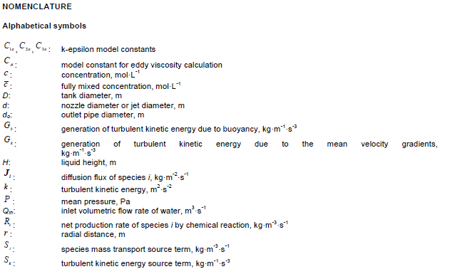
where Ï• is a universal dependent variable, U is mean velocity vector, Γφ is the diffusivity, and Sφ is the source term. The details of variable for continuity equation and momentum equations are expressed in Table 1. Generally, the values of eddy viscosity or turbulent viscosity (μt) in Table 1 are obtained by using turbulence fields.
Modeling of turbulence
The k-epsilon model includes two extra transport equations to represent the turbulent properties of the flow. The original model was proposed by Launder and Spalding (ANSYS Inc., 2013). Transport equations are resorted to resolving the turbulent kinetic energy (k) and the dissipation rate of turbulent kinetic energy (ε).
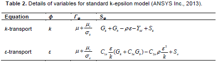
According to the general Reynolds average equation (Eq. (1)), the details of variables for standard k-epsilon model are expressed in Table 2. Furthermore, the model constants C1ε, C2ε, C3ε, σk, and σε are 1.44, 1.92, 0.09, 1.0, and 1.3, respectively (ANSYS Inc., 2013).
Modeling of species transport
In order to obtain the tracer concentration in the tank, the species transport equations without reaction were employed. In FLUENT, the general species transport equations (ANSYS Inc., 2013) can be written as
where Yi is the local mass fraction of species i, Ji is the diffusion flux of species i, Ri is the net rate of production of species i by chemical reaction, and Si is the source term of species transport equations.
Configuration of the jet mixing tank
The jet mixing tank was set up based on the previous work reported by Patwardhan and Gaikwad (2003). The details of eleven tested jet mixing tanks are given in Table 3.
Boundary conditions
A velocity inlet boundary condition was used at jet nozzle inlet, meaning that a velocity normal to the inlet was specified. The inlet velocity magnitude and turbulence intensity were 4.4 m·s-1 and 10%, respectively. A pressure outlet boundary condition was applied at the tank outlet. The symmetry boundary condition (no flow across the boundary and zero normal scalar flux) was adopted at the top of tank. At the wall, no-slip boundary condition was employed. The water density and water viscosity were 998.2 kg·m-3 and 0.001003 kg·m-1·s-1, respectively.
Numerical schemes
The pressure-velocity coupling of this simulation was SIMPLE, which stands for Semi Implicit Method for Pressure-Linked Equations. The numerical scheme for pressure was standard. For momentum, turbulence quantities, and mass species, the interpolation schemes were second order upwind. For unsteady state simulation, the transient formulation was first order implicit.
Investigation of mixing time
In experimental work of Patwardhan and Gaikwad (2003), the dilute NaCl was injected at the top liquid surface center. The four conductivity probes were employed to obtain the concentration distribution and mixing time. The four probes were located at different positions as shown in Figure 1. The mixing time was considered as the time required for the concentration (
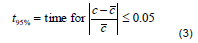
c) to reach within 95% of the fully mixed value (

). The mixing time (
t95%) can be decided by the following definition:
In this research, the tracer with a volume of 7.854 mL was injected at the center of top liquid surface. The properties of tracer and water were assumed to be identical. The concentrations of four different probes were monitored and used (Equation 3) to evaluate the mixing time for these probes. The longest mixing time was adopted to identify the mixing time in the tank.
Strategy of jet mixing tank simulation
This simulation was distinguished into two parts. First, the three-dimensional steady state was simulated to obtain the steady state flow field of water jet. Second, the three-dimensional unsteady state simulation was employed to achieve the concentration field of tracer in the tank. The average residence time in the tank was adopted to determine the time step size of unsteady simulation. The average residence time was calculated by using the inlet volumetric flow rate of water (Qin) and tank volume (V). The residence time, tres (tres = V / Qin ) of standard tank (S2) was 445.175 s. This value was employed to select the time step.
The time step size of the unsteady simulation should be a small fraction of the average residence time (Elsayed and Lacor, 2011, 2012). The small time step size is also conducted when the concentration gradient is large (Patwardhan, 2002). Moreover, Zughbi and Ahmad (2005) showed that the time step size of 1 s is sufficient to simulate jet mixing tank. So, in order to eliminate any uncertainty, the time step size of 0.0025 s was selected because it is very small as compared to the average residence time and the previous work of Zughbi and Ahmad (2005). The scaled residual of 10-5 was set to get the accurate results.
CFD grid
The jet mixing tanks and their grids were generated by using GAMBIT. The high grid density for these tanks was generated at the jet nozzle exit region. The grid generation of standard jet mixing tank (S2) is shown in Figure 2.
In order to eliminate the numerical uncertainty, the grid independent test has been applied to the standard jet mixing tank (S2). Four levels of grid for jet mixing tank, including 680,997, 737,707, 908,809, and 1,110,432 nodes, were studied. The jet centerline axial velocity profiles were compared and represented in dimensionless form as shown in Figure 3. The dimensionless velocity was defined as the ratio of jet axial velocity (v) to jet discharge velocity (Ujet). Furthermore, the dimensionless longitudinal jet distance was defined as the ratio of longitudinal jet distance (s) to jet diameter (d).
In Figure 3, it has been observed that the jet axial velocity of 680,997 nodes decay faster than the other grid levels. Moreover, the axial velocity profiles obtained by 737,707, 908,809, and 1,110,432 nodes are slightly different. However, in order to exclude any uncertainty, the simulations were performed using 908,809 nodes.
Validation of the model
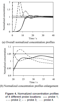
The standard jet mixing tank (S2) with 908,809 nodes was simulated by using standard k-epsilon turbulence model. The simulated results were compared with the previous work of Patwardhan (2002). The predicted concentration profiles of different probes were represented in dimensionless form as depicted in Figure 4. The normalized concentration was defined as the ratio of the local concentration to the well-mixed concentration.
In Figure 4, the 95% approach to the well-mixed concentration leads to different mixing time for different probe locations. The normalized concentration profiles of probe 1 and probe 4 are slightly different because their probe locations are symmetrical as shown in Figure 1.
Probe 3 represents the largest mixing time. In this study, the largest mixing time was adopted to identify the mixing time of the jet mixing tank. The predicted mixing time obtained by probe 3 and experimental mixing time are 26 s and 30 s, respectively. The error between simulation and experiment is 13.3%. This shorter predicted mixing time is due to an overprediction in the extent of turbulent dispersion. That is, the predicted turbulent diffusivity would be higher than experiment.
Further, the simulated normalized concentration profiles of probes 1 and 2 were compared with the two different previous CFD results (216,000 computation nodes), including the model with Cμ of 0.09 and C1ε of 1.44 (standard model constants) and the model with Cμ of 0.135 and C1ε of 1.31 (modified model constants), and the experimental data reported by Patwardhan (2002) as depicted in Figure 5. It can be seen that the present predicted normalized concentration profile of probe 1 are much closer to the experimental data than two different previous CFD results.
For probe 2, it can be observed that the CFD results during 0 to 14 s deviate from the experiment because the flat liquid surface with symmetry boundary condition was assumed. However, these simulated results of probe 2 approach the experimental data, at least, time after 20 s.
According to these results, it can be concluded that the prediction of normalized concentration profile can be improved by increasing number of nodes or decreasing the mesh size and using the second order upwind discretization scheme.
These results also referred that the poor predicted normalized concentration profiles obtained by previous studies may be due to the numerical errors rather than inadequacies in the standard k-epsilon turbulence model. Hence, this normalized concentration profile improvement method is more realistic than other methods because a good agreement between predicted normalized concen-tration profile and experimental data is observed without adjusting the model parameters (no longer fine tuning). Moreover, for mixing time, the agreement between simulation and experiment is acceptable. Thus, this simulation methodology is reasonably adopted to simulate the jet mixing tanks.
Effect of jet nozzle angle on mixing time
In order to investigate the effect of jet nozzle angle on mixing time for different liquid heights, the tanks with various ratios of liquid height (H) to tank diameter (D), including 0.5, 1, and 1.5, were simulated by varying the jet nozzle angle of 22.5º, 45º, and 67.5º, respectively. As reported by previous works, the mixing time was found to be inversely proportional to the jet path length (L) (Maruyama et al., 1982; Grenville and Tilton, 1997), which is defined as a distance between jet nozzle exit and tank wall or liquid surface, meaning that the higher jet path length results the shorter mixing time. It seems logical to define the jet path length as reported by previous works. However, this definition is only a geometric parameter, which is not an actual jet path length. Therefore, in this study, the jet stream lines of nine different tanks as shown in Figure 6 were directly employed to measure the jet path lengths. The jet path lengths were measured by the jet streamlines from the center of jet nozzle exit to the position where the streamlines hit the tank wall or top liquid surface. These jet path lengths were represented in dimensionless form, which defined as a ratio of jet path length to jet nozzle diameter, as shown in Table 4. Further, the details of these tanks, including ratio of H/D and nozzle angle, and their simulated mixing times were also summarized as shown in Table 4.
From Figure 6, the results revealed that the jet flow patterns depended on the jet nozzle angle and H/D ratio. Moreover, these jet streamlines ensured that these jets hit the opposite boundaries. In Table 4, it is showed that the mixing times are found to increase with increasing H/D ratio because the larger tank volume requires more jet energy and the tanks with nozzle angle of 45º show the smallest mixing time regardless of H/D ratios. Further, the L/d ratios of these tanks are less than 100.
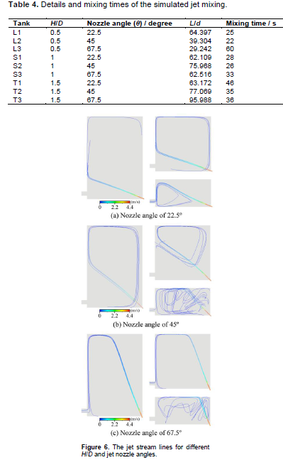
Generally, the surrounding fluid is entrained by jet within L/d of 400 (Harnby et al., 1997; Perona et al., 1998; Wasewar and Sarathi, 2008). These results ensured that the jets can entrain the external liquid and generate the circulation inside the tanks. When the mixing time and jet path length are viewed together, it can be seen that the mixing time of H/D of 1 shows inversely proportional to the jet path length. Whereas, the mixing times of other H/D ratios exhibit the different tendency, which contrast to the previous works (Maruyama et al., 1982; Grenville and Tilton, 1997).
In order to conceive the difference in the mixing time of these tanks, the axial velocities along the jet centerline for different tanks were measured and represented in dimensionless form as shown in Figure 7. The dimensionless jet centerline axial distance was defined as the ratio of the jet centerline axial distance (s), which was measured from the jet nozzle exit, to jet nozzle diameter (d).

In Figure 7, it can be observed that the dimensionless velocity profiles can be distinguished into two regions. The first region exhibits the constant dimensionless axial velocity, which is known as the zone of flow establishment (ZFE) or potential core (Seok and Il, 2005; Ball et al., 2012). The mixing in this zone is due to the large-scale coherent structures (CS), which is called bulk mixing (Wang and Keat Tan, 2010). The dimensionless velocity profiles of these H/D ratios are slightly different. These similar profiles for three different H/D ratios are observed because the results are measured near the jet exit region, where the boundary conditions are identical. These results can be implied that the jet velocity profiles near the jet nozzle exit region are not dependent on the liquid height.
Further, the simulated results revealed that the constant dimensionless velocities for nozzle angle of 45º (s/d ≈ 4) are larger than two other jet nozzle angles (s/d ≈ 2) for three different H/D ratios because of the freedom of jet flow, that is, the wall disturbance of the tanks with a nozzle angle of 45º are less than the two other nozzle angles. In the second region, the dimensionless velocities are found to decrease with increasing dimensionless longitudinal jet distance, which is called zone of established flow (ZEF) (Seok and Il, 2005). The smaller scale mixing of this region is driven by turbulent velocity fluctuations (Wang and Keat Tan, 2010). Moreover, it can be seen that the decay in dimensionless velocities profiles for nozzle angle of 67.5º are faster than the others because the jet kinetic energy is partly converted to potential energy.
When Table 4 and Figures 6 and 7 are viewed together the following observations can be drawn:
(i) The different nozzle angles dramatically exhibit the different flow patterns inside the tanks, such as potential core length, jet path length, jet centerline velocity profile, etc. Further, the different flow fields result in the different mixing times. In other words, the mixing time is dependent on flow pattern inside the tank.
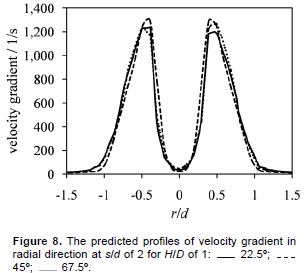
(ii) The tanks with nozzle angle of 45º exhibit the shortest mixing time because of their longest potential core zones or their largest mass entrainment. The largest mass entrainment for nozzle angle of 45º can be confirmed and investigated by considering the transverse profiles of jet axial velocity gradient in radial direction (dv/dr) as shown in Figure 8.
In Figure 8, it can be seen that, for -0.5 > r/d > 0.5, the velocity gradient for nozzle angle of 45º is about 10% lower than the others, meaning that the difference in momentum concentration (or mass flux) between inner zone of jet and jet boundary is smaller than two other nozzle angles. In other words, at jet boundary, the jet with 45º nozzle angle entrains more external fluid mass as compared to the others. Moreover, the higher mass entrainment in potential core also results in the higher mass entrainment in far field region (Gutmark and Grinstein 1999).
(iii) For the nozzle angles of 22.5º and 67.5º, it can be seen that the potential core lengths are identical and the longer jet path lengths result in the shorter mixing times. Further, the jet path lengths are slightly different as observed in the tank with H/D of 1, the higher jet centerline velocity (jet kinetic energy) yields the shorter mixing time.
Furthermore, in order to confirm the cause of the difference in mixing time for different tanks, the tanks with the diagonal nozzle angle were also tested. The mixing times and tank descriptions are shown in Table 5. Further the predicted dimensionless axial velocity profiles along the jet centerline are depicted in Figure 9.
From Table 5 and Figure 9, for H/D of 0.5, although the L/d ratio of diagonal jet angle tank is longer than the tank with nozzle angle of 45º, the mixing time of diagonal jet angle tank is larger than the 45º nozzle angle tank becuase of its shorter potential core length. Further, the potential core lengths of the tanks with diagonal jet angle and nozzle angle of 22.5º are identical. However, the tank with nozzle angle of 22.5º exhibits shorter mixing time because of its higher jet path length and centerline dimensionless velocity in zone of established flow.
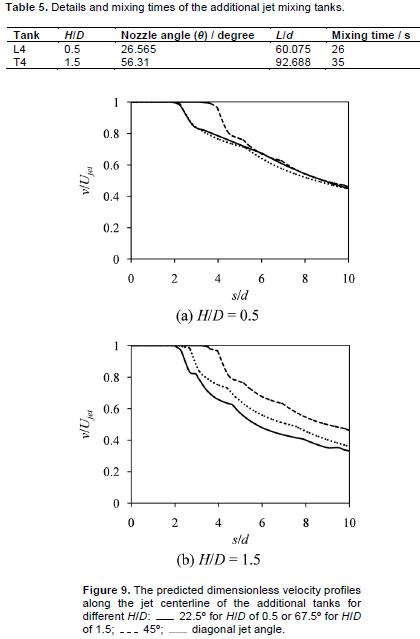
For H/D of 1.5, the mixing times of the tank with the diagonal jet angle and the tank with the nozzle angle of 45º are identical. While, the potential core length and L/d ratio of the tank with diagonal jet angle are, respectively, shorter and longer than that observed in the tank with nozzle angle of 45º. The mixing time of the tank with diagonal jet angle is identical to the tank with nozzle angle of 45º because the effective mixing in longer jet path length compensates for poor mixing in shorter potential core length. Moreover, the mixing time for diagonal jet is shorter than the tank with nozzle angle of 67.5º because of its longer potential core length.
Further, these results indicated that (i) When the potential core lengths were identical, the mixing time is dependent on jet path length or centerline jet velocity (jet kinetic energy). (ii) The mixing time of the tanks with short potential core length can be improved by changing the nozzle angle approach to 45º because the effect of wall disturbance on the jet is decreased.
According to these results, it can be summarized that the difference in mixing time is caused by the difference in jet flow pattern inside the tank, which is due to the different nozzle angles and H/D ratios. The shortest mixing time is achieved by the tank with nozzle angle of 45º because of the largest mass entrainment in potential core region. These results evidenced that the primary effect on mixing time is potential core zone. Moreover, the jet path length or jet centerline velocity (jet kinetic energy) is considered as the secondary effect on mixing time.
Comparison of previous reports
Here, the present simulated mixing times for H/D of unity were compared with the previous results of Patwardhan and Gaikwad (2003) and Zughbi and Ahmad (2005) for two different reasons. First, the experimental work of Patwardhan and Gaikwad (2003) is employed to demonstrate the jet mixing times in the tanks with identical power input through the jet nozzle (Pjet = πρd2Ujet3/8 ≈ 2.14 W). Second, the CFD work of Zughbi and Ahmad (2005) is adopted only to compare the difference in mixing time tendency between the jet mixing tank with top solid wall (the tank with nozzle angle of 45º shows the maximum mixing time) and the present open jet mixed tank (the tank with nozzle angle of 45º represents the minimum mixing time).
Due to the difference in tank volume, jet power, and jet Reynolds number of these works, only the tendency of the mixing time, not their values, was compared. The tank geometries of the present work and Patwardhan and Gaikwad (2003) are identical, except the jet nozzle diameter. The tank with top solid wall of Zughbi and Ahmad (2005) is smaller than the other tanks. The details of jet mixing tanks, conditions, and mixing times of the present and previous studies can be sumarized as shown in Table 6. Moreover, the mixing times of these works were plotted against the jet nozzle angle as shown in Figure 10.

In Table 6, the mixing times for differnt jet nozzle angles are found to decrease with increasing jet Reynolds number. These results confirm the previous studies that the mixing time is dependent on jet Reynolds number (Hiby and Modigell, 1978; Lane and Rice, 1981). Further, in Figure 10, the results of the present work and Pawardhan and Gaikwad (2003) revealed that the nozzle angle of 45º exhibits the minimum mixing time and the mixing times are decreased with incresing jet nozzle diameter, which is similar to the previous work of Patwardhan (2002).

In contrast, the mixing time for jet nozzle angle of 45º, which exhibits the longest jet path length, reported by Zughbi and Ahmad (2005) shows the maximum value. This result contradicts the suggestion that the longest jet path length results in the shortest mixing time (Maruyama et al., 1982; Grenville and Tilton, 1997). For the tank of Zaghbi and Ahmad (2005), the top of liquid height is bounded by a solid wall, which is different from the other tanks.
For this 45º tank, the jet diagonally flows through the tank and impinges on the opposite corner. Then, the jet loses its momentum and splits into two streams. These streams move and lose their momentum along the top and side walls. Further, these two weak streams generate poor circulation inside the tank. This flow phenomena indicated that the maximum mixing time of this 45º tank is due to the weak circulation. For other jet nozzle angles, the jet impinges on the opposite side or top wall and creates the stronger fluid circulation as compared to the tank with nozzle angle of 45º (Zaghbi and Rakib, 2004; Zaghbi and Ahmad, 2005). That is, for nozzle angle below 45º, more of fluid volume comes within the upper jet agitated zone.
Moreover, for nozzle angle more than 45º, there is a jet rollover after it hits the top wall. After rollover, the jet drives the liquid to move along the tank wall and agitates the bulk liquid. Hence, the mixing time of these tanks are shorter than that observed in the tank with nozzle angle of 45º.
In this work, the jet mixing tank is an open cylinder tank, which is similar to the experimental work of Patwardhan and Gaikwad (2003). The flow phenomenon inside the tank is somewhat similar to the tank of Zughbi and Ahmad (2005). However, the top liquid circulation is not limited by the solid wall, meaning that the top liquid motion does not lose its momentum due to the absence of the top solid wall.
The top liquid is easily re-entrained by the jet, which increases the effectiveness of the jet as a mixer. So, the concept of jet path length reported by Maruyama et al. (1982) and Grenville and Tilton (1997) is valid for this situation. As mentioned earlier, the tank with nozzle angle of 45º showed the shortest mixing time as compared to the other jet nozzle angles because of the longest jet path length and the longest potential core length.
According to these results, it can be summarized that the top solid wall reduces the effectiveness of the jet as a mixer. Further, the jet path length concept can be adopted only to describe the jet mixing time in the open tank. For the tank with top solid wall, the new definition of jet path length or new parameter should be defined to analyze the jet mixing time.
In this work, the CFD model was developed to study the effect of jet nozzle angle on mixing time for different H/D ratios. The simulated mixing time and concentration profiles were validated by comparing with the experiment and previous CFD models reported by Patwardhan (2002). The present model with 908,809 nodes exhibited an acceptable value of mixing time as comparing with the experiment. Further, this model successfully improved the accuracy of normalized concentration profile predictions by increasing the computational nodes, especially probe 1, as compared to the previous CFD models.
The nozzle angles of 22.5º, 45º, and 67.5º were employed to study the effect of jet nozzle angle on mixing time for different H/D ratios. The results revealed that the different nozzle angles are directly affected on the flow pattern inside the tanks and the mixing time. The tanks with nozzle angle of 45º exhibited the shortest mixing time regardless of H/D ratios because of their highest mass entrainment in potential core region. Further, the results indicated that the mixing time is mainly affected by the potential core length. The secondary effect on mixing time is the jet path length or jet centerline velocity (jet kinetic energy), which depend on the tank geometry.
The comparison between the present work and previous works indicated that the top solid wall reduces the effectiveness of jet mixer. Further, the concept of jet path length is only valid for the open jet mixing tank. In order to analyze the jet mixing tank with top solid wall, the new definition of jet path length or new parameter should be specified.
For future work, the large eddy simulation (LES) would be employed to predict these jet mixing tanks and compare the LES results with the results of k-epsilon model. Moreover, for the tanks with various H/D ratios, the future work would be directed towards employing the experiment to confirm these CFD simulated results.
The authors have not declared any conflict of interests.
The authors would like to thank Associate Professor Dr. Jarruwat Charoensuk, Department of Mechanical Engineering, Faculty of Engineering, King Mongkut's Institute of Technology Ladkrabang, Thailand for his ANSYS FLUENT 15.0 software support.
REFERENCES
|
ANSYS Inc. (2013). ANSYS Fluent Theory Guide (Release 15.0).
|
|
|
|
Baldyga J, Bourne JR, Zimmermann B (1994). Investigation of mixing in jet reactors using fast competitive–consecutive reactions. Chem. Eng. Sci. 49:1937-1946.
Crossref
|
|
|
|
|
Ball CG, Fellouah H, Pollard A (2012). The flow field in turbulent round free jets. Prog. Aerosp. Sci. 50:1–26.
Crossref
|
|
|
|
|
Coldrey PW (1978). Jet mixing. Industrial Chemistry Engineering Course. Paper. University of Bradford.
|
|
|
|
|
Elsayed K, Lacor C (2011). The effect of cyclone inlet dimensions on the flow pattern and performance. Appl. Math. Model. 35:1952-1968.
Crossref
|
|
|
|
|
Elsayed K, Lacor C (2012). The effect of the dust outlet geometry on the performance and hydrodynamics of gas cyclones. Comput. Fluids. 68:134-147. http://www.sciencedirect.com/science/article/pii/S004579301200298
Crossref
|
|
|
|
|
Fossett H (1951). The action of free jets in mixing of fluids. Trans. Inst. Chem. Eng. 29:322-332.
|
|
|
|
|
Fox EA, Gex VE (1956). Single-phase blending of liquids. AIChE J. 2:539-544.
Crossref
|
|
|
|
|
Ghahremanian S, Moshfegh B (2011). Numerical and experimental verification of initial, transitional and turbulent regions of free turbulent round jet. In: 20th AIAA Computational Fluid Dynamics Conference, Hawaii, AIAA pp. 2011-3697.
Crossref
|
|
|
|
|
Ghahremanian S, Moshfegh B (2014). Evaluation of RANS Models in Predicting Low Reynolds, Free, Turbulent Round Jet. J. Fluids Eng. 136(1):011201–1–011201–13.
Crossref
|
|
|
|
|
Grenville RK, Tilton JN (1996). A new theory improves the correlation of blend time data from turbulent jet mixed vessels. Chem. Eng. Res. Des. 74(A):390-396.
|
|
|
|
|
Grenville RK, Tilton JN (1997). Turbulence for flow as a predictor of blend time in turbulent jet mixed vessels. In: Nineth European Conference on Mixing, France, pp. 67-74.
|
|
|
|
|
Grenville RK, Tilton JN (2011). Jet mixing in tall tanks: Comparison of methods for predicting blend times. Chem. Eng. Res. Des. 89:2501-2506.
Crossref
|
|
|
|
|
Gutmark EJ, Grinstein FF (1999). FLOW CONTROL WITH NONCIRCULAR JETS. Annu. Rev. Fluid Mech. 31:239-272.
Crossref
|
|
|
|
|
Harnby N, Edwards MF, Nienow AW (1997). Mixing in the Process Industries. 2nd ed. Butterworth-Heinemann.
|
|
|
|
|
Hiby JW, Modigell M (1978). Experiments on jet agitation. In: 6th CHISA Congress, Prague.
|
|
|
|
|
Hoffman PD (1996). Mixing in a large storage tank. AIChE Symp. Ser. 286(88):77-82.
|
|
|
|
|
Lane AGC, Rice P (1981). An experimental investigation of liquid jet mixing employing a vertical submerged jet. IChemE Symp. Ser. 64. paperK1.
|
|
|
|
|
Lane AGC, Rice P (1982). An investigation of liquid jet mixing employing an inclined side entry jet. Trans. Inst. Chem. Eng. 60:171-176.
|
|
|
|
|
Maruyama T (1986). Jet mixing of fluids in vessels. Encyclopaedia of Fluid Mechanics Gulf Publishing Company Vol. 2.
|
|
|
|
|
Maruyama T, Ban Y, Mizushina T (1982). Jet mixing of fluids in tanks. J. Chem. Eng. Jpn. 15(5):342-348.
Crossref
|
|
|
|
|
Okita N, Oyama Y (1963). Mixing characteristics in jet mixing. Jpn. J. Chem. Eng. 31(9):92-101.
Crossref
|
|
|
|
|
Patwardhan AW (2002). CFD modeling of jet mixed tanks. Chem. Eng. Sci. 57:1307-1318.
Crossref
|
|
|
|
|
Patwardhan AW, Gaikwad SG (2003). Mixing in tanks agitated by jets. Trans. IChemE. 81(A):211–220.
Crossref
|
|
|
|
|
Paul EL, Atiemo-Obeng VA, Kresta SM (2004). Handbook of Industrial Mixing. John Wiley & Sons.
|
|
|
|
|
Perona JJ, Hylton TD, Youngblood EL, Cummins RL (1998). Jet Mixing of Liquids in Long Horizontal Cylindrical Tanks. Ind. Eng. Chem. Res. 37:1478-1482.
Crossref
|
|
|
|
|
Schimetzek R, Steiff A, Weinspach PM (1995). Examination of discontinuous jet mixing for designing emergency cooling systems of chemical reactors. ICEME Symp. Ser. 136:391-398.
|
|
|
|
|
Seok JK, Il WS (2005). Reynolds number effects on the behavior of a non-buoyant round jet. Exp. Fluids 38:801-812.
Crossref
|
|
|
|
|
Simon M, Fonade C (1993). Experimental study of mixing performances using steady and unsteady jets. Can. J. Chem. Eng. 71:507-513.
Crossref
|
|
|
|
|
Wang X, Keat Tan SK (2010). Environmental fluid dynamics-jet flow. J. Hydrodyn. 22(5):1009-1014.
Crossref
|
|
|
|
|
Wasewar KL, Sarathi JV (2008). CFD modelling and simulation of jet mixed tanks. Eng. Appl. Comp. Fluid. 2(2):155-171.
Crossref
|
|
|
|
|
Zughbi HD, Rakib MA (2004). Mixing in a fluid jet agitated tank: effects of jet angle and elevation and number of jets. Chem. Eng. Sci. 59:829-842.
Crossref
|
|
|
|
|
Zughbi HD, Ahmad I (2005). Mixing in Liquid-Jet-Agitated Tanks: Effects of Jet Asymmetry. Ind. Eng. Chem. Res. 44:1052-1066.
Crossref
|
|