Full Length Research Paper

ABSTRACT
The use of yield-level management zones (MZs) has demonstrated high potential for site-specific management of crop inputs in traditional row crops. Two approaches were use: all variables approach (all_Var) and stable variables approach (sta_Var). In each approach, variables selected had significant correlation with yield, while all redundant and non-autocorrelated variables were discarded. Two fields were use in this study: Field 1 (17.0 ha soybean field located in Cascavel, Paraná, Brazil); and Field 2 (35.0 ha corn field located in Wiggins, Colorado, US.). Two, three, four, and five MZs were created using fuzzy c-means clustering technique. The proposed methodology for define MZs is simple and allowed create good-quality MZs. It also founded that not-stable-over-time variables are not useful to define MZs.
Key words: Precision agriculture, spatial variability, fuzzy clustering, autocorrelation, cross-correlation.
INTRODUCTION
A management zone (MZ) is a sub-region of a field that expresses a relatively homogeneous combination of yield-limiting factors for which a single rate of a specific crop input is appropriate (Doerge, 1996). Delineation of MZs and management of crop inputs have proved economical for application of variable rate inputs (Koch et al., 2004). Several researchers have successfully used one or more of these factors in combination with yield maps and sometimes use only multiple year yield maps in delineating MZs (Blackmore, 2000; Fraisse et al., 2001; Johnson et al., 2003; Schepers et al., 2004).
Numerous approaches are presented in literature for purpose of delineating MZs using yield maps, using cluster analysis, such as K-means and Fuzzy C-means (Taylor et al., 2007; Li et al., 2007). Although several techniques have been developed to delineate MZs, only few studies compared MZs in terms of their accuracy (Hornung et al., 2006). The following cluster performance indices can be used:
1. Variance reduction (VR; Ping and Dobermann, 2003; Xiang et al., 2007)
2. Fuzziness performance index (FPI); and
3. Modified partition entropy index (MPE; Fridgen et al., 2004). To evaluate the quality of the cluster process, two analyses could be conducted:
The average comparison test (analysis of variation, ANOVA; Bazzi et al., 2015)
Smoothness index (SI; Schenatto et al., 2016), which is a measure of the smoothness of the contour curves.
Although a careful definition of MZs requires a lot of steps and analysis about data. The goal of this study was to analyze viability of MZs definition using stable and non-stable variables and use methodology to define best number of zones for each case. This would be very interesting for producers who are only starting to use precision agriculture.
MATERIALS AND METHODS
Study site and data collection
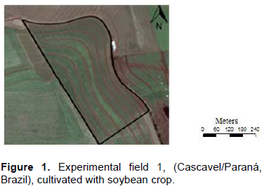
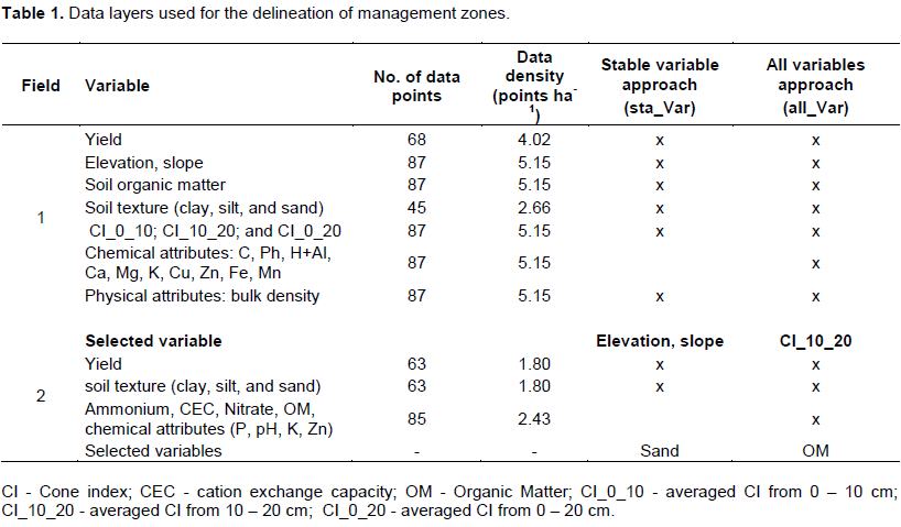
Field 1: Data from a 16.9 ha soybean field (Figure 1) were evaluated. It is located in a rural area of municipality of Cascavel, Paraná state, Brazil (24°57ʹ13ʺS and 53°34ʹ02ʺW, average elevation: 650 m). The soil is classified as distroferric red latossol (Embrapa, 1999) with 70% clay. A Trimble Geo Explorer XT 2005 Geodesic Differential Global Positioning System (GDGPS) with post-processing was used for georeferencing the research area. Soil samples (n = 87) were irregularly spaced throughout field. The following soil attributes were measure:
1. Soil texture (clay, silt, and sand)
2. Cone index (0 to 10 cm, CI_0_10; 10 to 20 cm, CI_10_20; and 0 to 20 cm, CI_0_20)
3. Chemical attributes: organic C, pH, Ca, and Mg, P and K, Cu, Zn, Fe, and Mn, and H+Al; and
4. Physical attributes: bulk density. The methodology from Embrapa (2009) was used to measured these variables. These attributes were used to define management zones because they have influence with potential yield to corn and soybean crops. Numerous researches were used for these attributes to define management zones, such as, Blackmore (2000), Fraisse et al. (2001), Johnson et al. (2003), Schepers et al. (2004), Taylor et al. (2007) and Li et al. (2007).
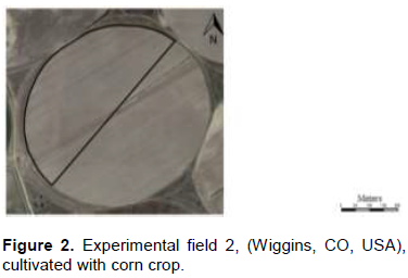
Field 2 (Figure 2) was approximately 35 ha in size and was nearly level (0 to 2% slope), with an average elevation of 1437 m. The area was cultivated with corn and is located in the rural area of the municipality of Wiggins, Colorado, USA (40°19ʹ59ʺN and 104°01ʹ50ʺW). The dominant soil types were Valentine fine sand (mixed, mesic, Typic Ustipsamment) and Dwyer fine sand (mixed, mesic, Ustic Torripsamment) series (USDA, 1986). The following soil attributes were measure: soil texture (clay, silt, and sand); ammonium; cation exchange capacity (CEC); nitrate; organic matter (OM); and chemical attributes (P, pH, K, Zn).
Exploratory analysis and data interpolation
Exploratory analysis was apply to characterize variability in soil data with coefficient of variation (CV). The Anderson–Darling and Kolmogorov–Smirnov tests applied to test normality data at 0.05 significance level. Potential outliers were identify using box-plots. Inverse distance weighting (IDW) was apply to interpolate field data. IDW was choose because of its simplicity, and successful results of interpolation of field data have been reported (Jones et al., 2003). A leave-one-out cross-validation applied to identify number of neighbors and exponent distance used in interpolation of each variable. For this methodology, a routine was write using software R.
Spatial correlations
Moran’s bivariate spatial autocorrelation statistics (Czaplewski and Reich, 1993) were apply to assess spatial correlation between analyzed attributes and to establish spatial correlation matrix. This matrix checks and identifies attributes that influence yield positively or negatively, and checks if a sample was correlate spatially (spatial autocorrelation). The attributes used in the generation of MZs were selected by the variable selection method proposed by Bazzi et al. (2013):
1. Elimination of variables with non-significant spatial correlation at 5% probability level
2. Elimination of variables that had no spatial correlation with yield
3. Ordering variables according to the degree of spatial correlation with yield; and
4. Elimination of redundant variables (that are spatially correlated with each other), giving preference to the maintenance of variables that have a higher correlation with yield.
Delineation of management zones
Clustering methods are appropriate for dividing data into groups with homogeneous characteristics. Of these, the Fuzzy C-Means is used most often (Li et al., 2007; Fu et al., 2010; Zhang et al., 2013; Li et al., 2013; Moral et al., 2010). This algorithm uses a weighting exponent to control the degree of sharing between classes (Bezdek, 1981), allowing individuals to exhibit partial adhesion in each of the classes, which is important when dealing with the continuous variability of natural phenomena (Burrough, 1989).
Usually only those attributes that do not vary appreciably over time as chemical attributes are used to create MZs that are intended for use for many years (Doerge, 1996). However, for special conditions, MZs are use for nutrients and lime application in the following year. Chemical attributes may be included as MZ attribute variables. Two approaches were apply to delineate MZs: all variables approach (all_Var) and stable variables approach (sta_Var). In the first approach, variables with a significant spatial cross-correlation with the yield were select to delineate MZs. The selected variables may or may not be stable over time. In sta_Var, only those variables that were stable over time (Table 1) and spatially cross-correlated with the yield (Doerge 1996) were consider for delineation MZs (Table 1).
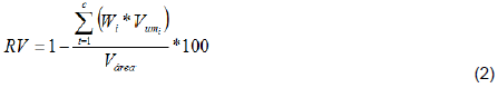
Two to five MZs were created using interpolated data and fuzzy c-means clustering; for this purpose, Software for Defining Management Zones (SDUM; Bazzi et al., 2013). Each variable was standardize according to Eq. 2 prior to clustering:
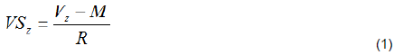
where: is the value of the standardized variable at the spatial location of position
  is the value of the original variable at the spatial location of z; M is the median; and R is the range of the data (Mielke and Berry, 2007).
Evaluation of management zone delineation
Variance reduction (VR; Equation 2; Xiang et al., 2007):
where c is the number of MZs;  the proportion of the area in each MZ;
 the variance of the sample data of each MZ; and
  the variance of the sample of the data for the entire field.
Fuzziness Performance Index (FPI; Equation 3; Fridgen et al., 2004)
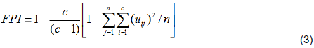
where c is the number of clusters; n, the number of observations; uij, the element of the fuzzy membership matrix.
Modified partition entropy (MPE; Equation 4; Boydell and Mcbratney, 2002)
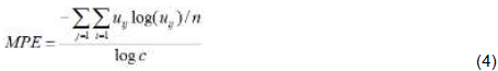
where c is the number of clusters; n, the number of observations; and  , the ij-th elements of the fuzzy membership matrix.
RESULTS AND DISCUSSION
Descriptive statistics
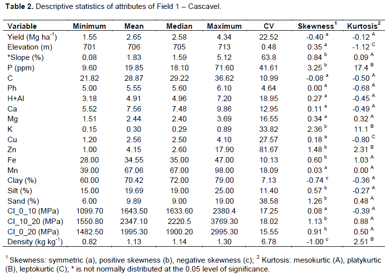
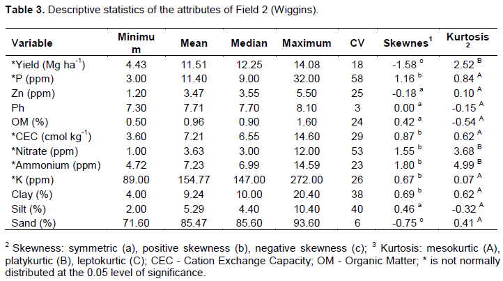
The descriptive statistics for selected attributes of Field 1 are indicated that all variables, except for slope, were it isnormally distributed (Table 2). Most variables showed symmetric and mesokurtic distributions. The CV was low for elevation, pH, bulk density, and clay; medium for Fe, C, silt, Ca, cone index (0 to 10 cm, CI_0_10; 10 to 20 cm, CI_10_20; and 0 to 20 cm, CI_0_20), Mg, Mn, and H+Al; high for the yield and Cu; and very high for K, sand, P, the slope, and Zn. In case of Field 2 (Table 3), clay, silt, sand, OM, pH, and Zn were normally distributed. The CV was low for the pH and sand; medium for yield; high for Zn, OM, CEC, ammonium, and K; and very high for P, nitrate, clay, and silt.
Spatial autocorrelation and cross-correlation
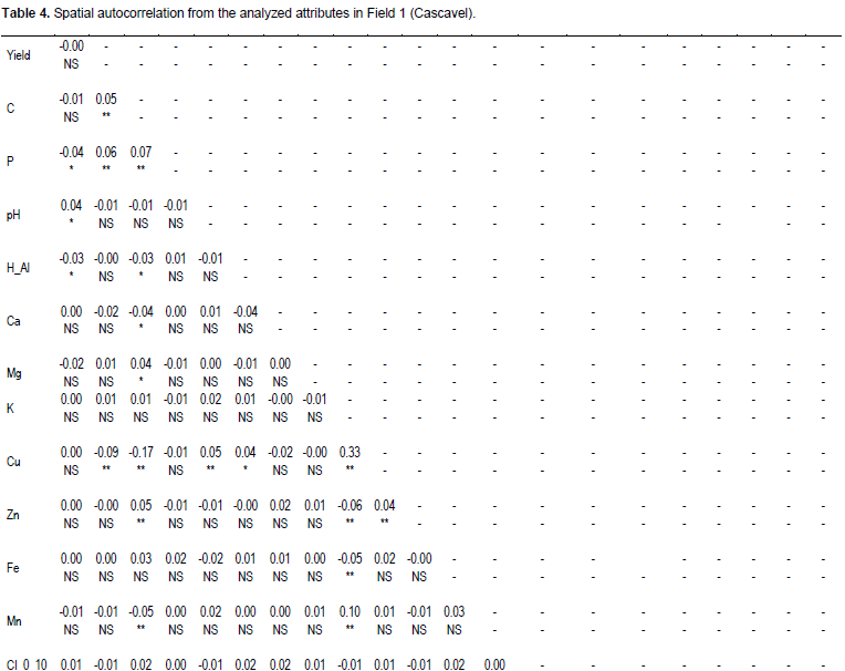
The attributes analyzed values for Field 1 were show at Table 4. Variables Cu, clay, elevation, CI_10_20, CI_0_20, sand, slope, P, C, Zn, and bulk density had significant positive autocorrelations. Variables CI_10_20, elevation, CI_0_20, bulk density, slope, sand, clay, silt, pH, P, and H+Al were significantly cross-correlated with yield. Bazzi et al. (2013) found a high correlation between soybean yield with soil sand percentage, generating agricultural area MZs with this layer. Similarly, Schenatto et al. (2016), Peralta and Costa (2013) and Gavioli et al. (2016) generated MZs from elevation data and CI in experimental soybean and cornfields.
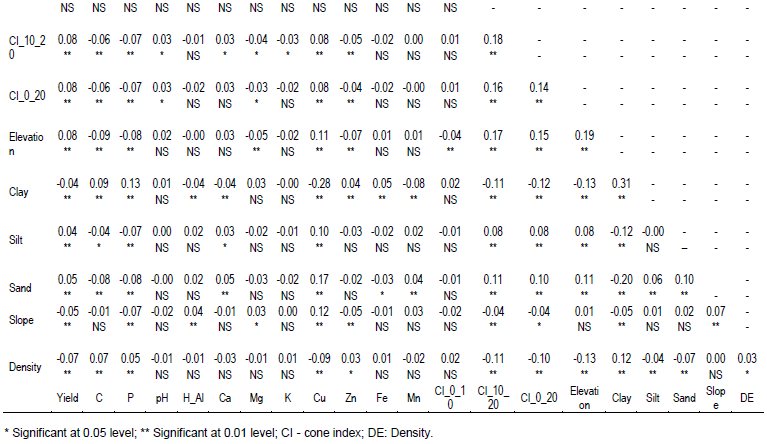
The values for Field 2 were show in Table 5. Variable yield, P, nitrate, Zn, CEC, OM, K, clay, sand, silt, and ammonium exhibited significant autocorrelations. Variables OM, CEC, sand, NH3, clay, K, silt, and Zn were significantly cross-correlated with the yield. Other studies yielded similar results: for example, Bansod and Pandey (2013) and Jaynes et al. (2003) identified high correlation between CEC and yield.
Management zones
Figure 3 shows the MZs as a function of zone number (from two to five) and approach (sta_Var and all_Var) for Field 1 (Cascavel) and Field 2 (Wiggins). In all cases, this can be see when the number of zones increased, the amount of fragments of the area is bigger.
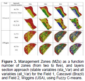
For Field 1, data layers selected to delineate MZs using sta_Var (approach) were elevation and slope, whereas MZs based on all_Var based on CI_10_20. CI_10_20 was not selected as sta_Var because it was not stable over time. However, because it showed highest spatial correlation with yield and was cross-correlated with elevation and slope, it was included in all_Var selection. In this sense, in the lower areas, soybean yield was lower probably because rainfall was higher than average during cultivation, which may have resulted in excessive water in soil (Fausey, 1999). For Field 2, MZs based on sta_Var approach were delineated using sand, whereas in all_Var approach, OM used it. As in Field 1 case, OM was not select as sta_Var because it was not stable over time. In both approaches, selected correlated layers (sand and OM) were negatively spatially correlate with yield. In addition, sand and OM were correlate to CEC, meaning that this variable used to define MZs if sample and analysis costs were prohibitive.
The average yields differed significantly between two MZs (Table 6) in both fields. With three, four, and five zones only for Field 2, the average yields differed significantly. From these results and those reported by Zhang et al. (2013), it can be seen that the division of the area into two MZs was adequate for producing zones with different yields.
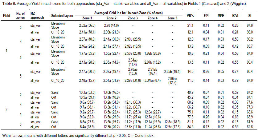
The VR of an MZ indicates whether MZ delineation is more efficient than having no MZs on field. In all cases (Table 6 and Figure 4), VR values were positive, indicating that in all cases, total variance reduced, as expected. In case of Field 1, VR remained reasonably constant with MZs number. However, in Field 2 case, VR increased with MZ number. The VR results confirm ANOVA results because it turns out that divisions within each zone did not show much variance from average, indicating regions of similar productive potential. These results corroborates those obtained by Xiang et al. (2007) and indicated that when divisions are satisfactory, VR tends to increase despite an increase in MZs number because there is smaller variation within each zone.
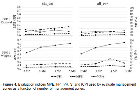
ANOVA shows for Field 1, that best division was two MZs (for sta_Var and all_Var) and up to five MZs for Field 2 (sta_Var and all_Var) (Table 6). The FPI, MPE, and VR indices (Figure 4) were also evaluated; smaller FPI and MPE, shows better clustering test for both fields, considering FPI and MPE. Best efficiency was obtain with two MZs, but best option with VR was two (sta_Var) and three (all_Var) MZs for Field 1 and five MZs for Field 2 (sta_Var and all_Var).
Two approaches comparison (sta_Var and all_Var) for two MZs (selected as best number of MZs) showed that sta_Var provides better VR. That means there is no meaning of using all variables (time stable or not) in defining MZs. The sta_Var MZs (with two MZs) presented a reduction in variance from 21 (Field 1) to 50% (Field 2). Because the MZ definition through Fuzzy c-means does not use variable yield only if several years’ yields could find other important and not redundant variable, the MZs would be same.
CONCLUSIONS
The methodology proposed for MZs define has practical value and allowed MZs definition with good quality. This results may be confirmed on the analysis of the variance reduction and Anova. For divisions in two zones (best division by MPE and FPI indexes), the variance reduction and Anova showed have different yield potential in each zone when the fields were divided. The stable variables approach performed better than all variables in all cases because they showed better results on the analysis from variance reduction and Anova, indicating that stable variables have influence in the yield capacity and can be used to define management zones that must be used for a long time. The stable variables approach also served as the source of recommendation and soil analysis and pre-plant or in-season fertilizer recommendation for precision agriculture.
CONFLICTS OF INTERESTS
The authors have not declared any conflict of interests.
ACKNOWLEDGMENTS
The authors are grateful to State University of Western Paraná (UNIOESTE), Technological Federal University of Paraná (UTFPR), Araucária Foundation (Fundação Araucária), Coordination for Improvement of Higher Education Personnel (CAPES), and National Council for Scientific and Technological Development (CNPq) for support received and for Agassis Linhares, agronomist engineer, for assignment of research area.
REFERENCES
|
Bansod BS, Pandey OP (2013). An Application of PCA and Fuzzy C-Means to Delineate Management Zones and Variability Analysis of soil. Eur. Soil Sci. 46(5):556-564. |
|
|
Bazzi CL, Souza EG, Konopatzki MRS, Nóbrega LHP, Uribe-opazo MA (2015). Management zones applied to pear orchard. JFAE 13(1):86-92. |
|
|
Bazzi CL, Souza EG, Opazzo MA, Nobrega LH, Rocha DM (2013). Management Zones definition using soil chemical and physical attributes in a soybean area. Eng. Agríc. 33(5):952-964. |
|
|
Bezdek CJ (1981). Pattern recognition with fuzzy objective function algorithms. New York: Plenum Press. |
|
|
Blackmore S (2000). The interpretation of trends from multiple yield maps. Comput. Electron. Agric. 26(1):37-51. |
|
|
Boydell B, Mcbratney AB (2002). Identifying potential within-field management zones from cotton yield estimates. Precision Agric. 3(1):9-23. |
|
|
Brazilian Agricultural Research Company [EMBRAPA] (1999). Brazilian System of Soil Classification. National Center for Soil Research. Rio de Janeiro, Brazil. (in Portuguese). |
|
|
Brazilian Agricultural Research Company [EMBRAPA] (2009). Manual chemical analysis of soils, plants and fertilizers. Rio de Janeiro, Brazil (in Portuguese). |
|
|
Burrough PA (1989). Fuzzy mathematical methods for soil survey and land evaluation. J. Soil Sci. 40(3):477-492. |
|
|
Czaplewski RL, Reich RM (1993). expected value and variance of moran bivariate spatial autocorrelation statistic for a permutation test. usda forest service rocky mountain forest and range experiment station research paper, (RM-309):1. |
|
|
Doerge T (1996). Management Zone Concepts. Site-Specific Management Guidelines Retrieved 19 March 2009. |
|
|
Evans RO, Fausey NR, Skaggs RW, Schilfgaarde JV (1999). Effects of inadequate drainage on crop growth and yield. Agric. Drain. 13-54. |
|
|
Fraisse CW, Sudduth KA, Kitchen NR (2001). Delineation of site–specific management zones by unsupervised classification of topographic attributes and soil electrical conductivity. T ASAE 44(1):155-166. |
|
|
Fridgen JJ, Kitchen NR, Sudduth KA, Drummond ST, Wiebold WJ, Fraisse CW (2004). Management zone analyst (MZA): software for subfield management zone delineation. Agron. J. 96(1):100-108. |
|
|
Fu Q, Wang Z, Jiang Q (2010). Delineating soil nutrient management zones based on fuzzy clustering optimized by PSO. Math. Comput. Mod. 51(11-12):1299-1305. |
|
|
Gavioli A, Souza EG, Bazzi CL, Guedes LPC, Schenatto K (2016). Optimization of management zone delineation by using spatial principal components. Comput. Electron. Agric. 127(1):302-310. |
|
|
Hornung A, Khosla R, Reich RM, Inman D, Westfall DG (2006). Comparison of Site-Specific Management Zones: Soil-Color-Based and Yield-Based. Agron. J. 98(1):407-415. |
|
|
Jaynes DB, Kaspar TC, Colvin TS, James DE (2003). Cluster analysis of spatiotemporal corn yield patterns in an Iowa field. Agron. J. 95(1):574-586. |
|
|
Johnson CK, Mortensen DA, Wienhold BJ, Shanahan JF, Doran JW (2003). Site-specific management zones based on soil electrical conductivity in a semiarid cropping system. Agron. J. 95(1):303-315. |
|
|
Jones NL, Davis RJ, Sabbah W (2003). A comparison of three-dimensional interpolation techniques for plume characterization. Ground Water 41(4):411-419. |
|
|
Koch B, Khosla R, Frasier M, Westfall DG, Inman D (2004). Economic feasibility of variable rate nitrogen application utilizing site-specific management zones. Agron. J. 96(6):1572-1580. |
|
|
Li Y, Shi Z, Wu H, Li F, Li H (2013). Definition of management zones for enhancing cultivated land conservation using combined spatial data. Environ. Manag. 52(1):792-806. |
|
|
Li Y, Zhoufeng SL, Hong-yi L (2007). Delineation of site-specific management zones using fuzzy clustering analysis in a coastal saline land. Comput. Electron. Agric. 56(2):174-186. |
|
|
Mielke PWJ, Berry KJ (2007). Permutation methods: a distance function approach. 1nd Ed. New York, USA, Springer. |
|
|
Moral FJ, Terrón JM, Silva JRM (2010). Delineation of management zones using mobile measurements of soil apparent electrical conductivity and multivariate geostatistical techniques. Soil Till. Res. 106(2):335-343. |
|
|
Peralta NR, Costa JL (2013). Delineation of management zones with soil apparent electrical conductivity to improve nutrient management. Comput. Electron. Agric. 99(1):218-226. |
|
|
Ping JL, Dobermann A (2003). Creating spatially contiguous yield classes for site-specific management. Agron. J. 95(5):121-113. |
|
|
Schenatto K, Souza EG, Bazzi CL, Bier VA, Betzek NM, Gavioli A (2016). Data interpolation in the definition of management zones. Acta. Sci. Technol. 38(1):31-40. |
|
|
Schepers A, Shanahan JF, Liebig MA, Schepers JS, Johnson SH, Luchiari A (2004). Appropriateness of management zones for characterizing spatial variability of soil properties and irrigated corn yields across years. Agron. J. 96(1):195-203. |
|
|
Taylor JA, Mcbratney AB, Whelan BM (2007). Establishing Management Classes for Broadacre Agricultural Production. Agron. J. 99(5):1366-1376. |
|
|
USDA-SCS (1986). Classification and correlation of the soils of Coastal Plains Research Center, ARS, Florence, South Carolina. USDA-SCS, South National Technical Center, Ft. Worth, TX. |
|
|
Xiang L, Yu-chun P, Zhong-qiang G, Chun-jiang Z (2007). Delineation and Scale Effect of Precision Agriculture management zones using yield monitor data over four years. Agric. Sci. China 6(2):180-188. |
|
|
Zhang Z, Lü X, Chen J, Feng B, Li XW, Li M (2013). Defining agricultural management zones using Gis techniques: Case study of Drip-irrigated cotton fields. Inf. Technol. J. 12(21):6241-6246. |
|
Copyright © 2024 Author(s) retain the copyright of this article.
This article is published under the terms of the Creative Commons Attribution License 4.0


