This study tries to tackle the tourism forecasting problem using online search queries. This recent-developed methodology is subject to several criticisms, one of which is how to choose satisfying search queries to be built in the forecasting model. This study compares two popular candidates, which are the Bayesian Model Averaging (BMA) approach and the Least Absolute Shrinkage and Selector Operator (Lasso) approach. Evidence shows that the two approaches produce similar forecasting performance but different query selection results.
In recent years, much attention on forecasting based on user generated content (UGC) has been paid. One representative is the data from search engine services. The users of search engines search certain key words, or queries, to acquire some information on purpose, which leaves the service providers a new route to analysis users' motivation and information demand.
In addition to these analyses, forecasting on certain issues can be conducted. A typical example is the Google Flu Trends (GFT), initialized in 2008, which has made several successful forecasts of flu outbreaks in US. The first paper on this issue is Ginsberg et al. (2009).
However, GFT is not as successful as it was initialized, and it has gone through many criticisms. Those criticisms come from the worries about the uncertainties of the query data generation process (DGP) and the model
instability (Butler, 2013) for example. Nevertheless, the forecasting on other aspects based on query data still contributes knowledge to both practitioners and academia, for example in tourism forecasting (Bangwayo-Skeete and Skeete, 2015; Yang et al., 2015; Li et al., 2017). The difference of the performance in different areas using search query data emerges partially from the variable selection approaches and forecasting models.
In most research, variable selection procedures based on correlation coefficient, purely subjective index compositing or other criteria might be problematic. Several researches try to improve the forecasting model by introducing variable selection models, such as spike and slab (Scott and Varian, 2014) and other pioneer approaches. As pointed by Brynjolfsson et al. (2015),successful forecasting based on query data has several problems to be settled, one of which is to solve the variable selection problem.
This study employed two frequently-used models with variable selection property to build the forecasting model on tourists forecasting. They are the Bayesian Model Averaging (BMA) approach and the Least Absolute Shrinkage and Selector Operator (Lasso) approach. Lasso is first proposed by Tibshirani (2011), and has many successful variants in predicting genome, economic amounts etc. BMA is sufficiently described in Hoeting et al. (1999), and it also has several follow-up updates.
In general, the two approaches can both select variables and conduct forecasting; however the mechanisms are totally different. The BMA approach, presumably, believes uncertainties exist in each model. Instead of choosing the best model, it advocates to combine those top models selected through Bayesian Factor or other criteria. Lasso applies soft-thresholding by introducing a penalty on model parameters when minimizing its squared error objective. Due to the different originalities of the two approaches, the theoretical comparison becomes extremely hard and, even, trivial.
However, from a practitioner's point of view, choosing between the two approaches is extremely useful. Except for the forecasting performance, the best model sizes and which variables are selected through BMA and Lasso also contribute to the forecasting practitioners.
Forecasting models
This section is to recap the main specification of the Bayesian Model Averaging (BMA), Least Absolute Shrinkage and Selector Operator (Lasso). Without loss of generality, we assume the underlying true model is of linear form, as shown in Equation 1:
where is the constant, X contains K covariates with N observations, and is the vector. Besides, in this model, we assume homoscedastic standard errors. Based on this specification, we now discuss the main results of BMA and Lasso.
Bayesian model averaging
To allow model uncertainties, we rearrange model (1) as
with as the model index, where . Each model of (2) in the Bayesian framework requires assumptions on priors of coefficient parameters

and variance

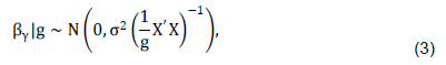
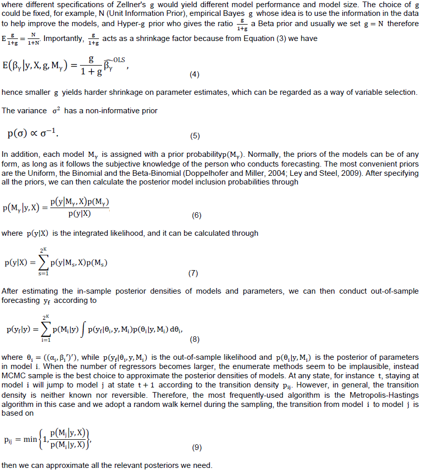
. Following the tradition assumption, (Feldkircher, 2012; Moral-Benito, 2015), we assume
follows a normal distribution with parameter Zellner's

in Feldkircher (2012):
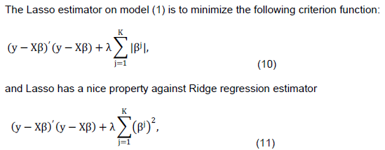
is that Lasso exhibit hard threshoding property which can rule out some irrelevant variables stricter than Ridge estimator.
Commonly, to guarantee the model stability of Lasso such that we can also mitigate model uncertainty to some degree, we apply cross-validation. Basically, we divide the sample into

subsamples. By taking

out of
subsample we estimate Lasso and take the rest one to compute the prediction errors. Then taking the average of the results, we can have a more stable forecasting model. In the empirical part, we choose to split the sample into 10 subsamples.
Notably, one might argue that the analysis here might be problematic since the time series structure could be destroyed during the cross-validation. However, the cross-validation here is not simply resampling over the original sample, instead block sampling methods are employed to keep the time series structure. Moreover, to have a more fair comparison, this paper does not expand the model into ARIMA or other popular time series models, since the introduction of lags might offset the true effects from the queries. The extension could be made in the future, and model (1) can be extended to any desired form, while this paper only contributes a benchmark.
Data collection
We collect the daily tourist records from a five-star resort, Jiuzhaigou, in Sichuan province in China. The reason why we choose this resort is that this resort is a perfect representative of those resorts attracting considerable amount of tourists everyday, and it has stably long-run inputs than any other new started resorts. In addition, compared to other resorts, the data it has is well-recorded, thus the data quality can be guaranteed.
The corresponding search query data is collected from a search engine website, provided by a dominant search engine service supplier, Baidu, in China. This company takes huge market shares so that the sample selection bias, on an aggregated level, is mitigated than any other data sources. We collect the data using an enumerate manner, namely we first pick several representative queries by our subjective knowledge and then take the recommended queries from the recommendation system of the search engine. Once either few new queries are recommended or the new words are totally irrelevant from our subjective knowledge, we stop iterating.
Finally, we have 148 relevant queries as candidates as indicators for forecasting. The queries collected reflect numerous demands on the tours to Jiuzhaigou, as summarized in the following categories: the name of the resort and its relevant information, the detailed information on the scenes inside the resort, the travelling information regarding the plans, suggestions, routes and other resorts nearby etc. Since the queries are in Chinese, in which the forming of words are quite different from English, we code each of them into an English category plus a number as an identifier. For example, the fifth query about travel information is coded as”TravelInformation5”. It can be seen that some queries are intuitively important since most of the travellers will search them while some queries recommended by the website are not a must for travellers to search. Subjective selection of queries become invalid given huge amount of candidate queries.
Therefore, it is needed to employ variable selection models to select the proper queries. Currently, we collect both the actual tourists records and the search query data from the 1st of June, 2012 to the 31th of August, 2014, with 822 observations on a daily basis.
Empirical comparisons
This section shows the comparisons of forecasting performance and variable selection between BMA and Lasso. For the BMA models, the forecasting performance evaluation is based on the posterior means of the predicted tourist amounts in the out-of-sample evaluation. For the Lasso, we apply 10-folded cross-validation method, and use the best model to do out-of-sample evaluation. For the stability of the results, the evaluation of each model takes the average of 5 times evaluations. Compared to Lasso, some details of BMA are given, because the basic settings of BMA are much flexible than Lasso which only has one tuning parameter

. Even though the Lasso is of simpler form, we also estimate Ridge estimator as a contrast.
To conduct this, we will consider the effects of different model priors, different MCMC sampling methods and different Zellner's
s. Since the Zellner's

acts as a shrinkage element which is viewed as the most important feature of BMA models, in the following empirical parts we first compare the models with different model priors and MCMC methods, then choose the best model featuring different Zellner's
to compare with Lasso.
Therefore after this short introduction, we then discuss the forecasting performance and the variable selection, and some estimate results of both BMA and Lasso are given prior to the comparison.
Model estimates
Before conducting the comparison, we first give some model estimates to have some straightforward ideas about the models involved, including the posterior inclusion probabilities of BMA models with different model priors, the quality of different MCMC methods and the shrinkage results of Lasso compared with Ridge estimator.
BMA estimates
We first estimate the BMA models. Since the performance model priors might be sensitive to the model's prior, that is

, we employ three different model priors to be compared for robustness, that is, uniform prior, binomial prior, and the beta-binomial prior. In addition, to avoid the case where certain MCMC sample is not effective in this particular research, we employ both the birth-death sampler and the reversible-jump sampler (Madigan et al., 19
In simple words, the birth-death sampler, in each round, randomly pick a variable to drop or to add, depending on whether the chosen variable is in the current model or not. The reversible-jump sampler assigns birth-death method a probability of 50% and for the other 50%, it swaps one of the variables already in the model with another one which is not in the current model. Importantly, the posterior mean of each parameter estimate is the weighted average across the top 200 models. To be noticed, if a variable is not included in a certain model, the coefficient, that is, zero, is also accounted into this average.
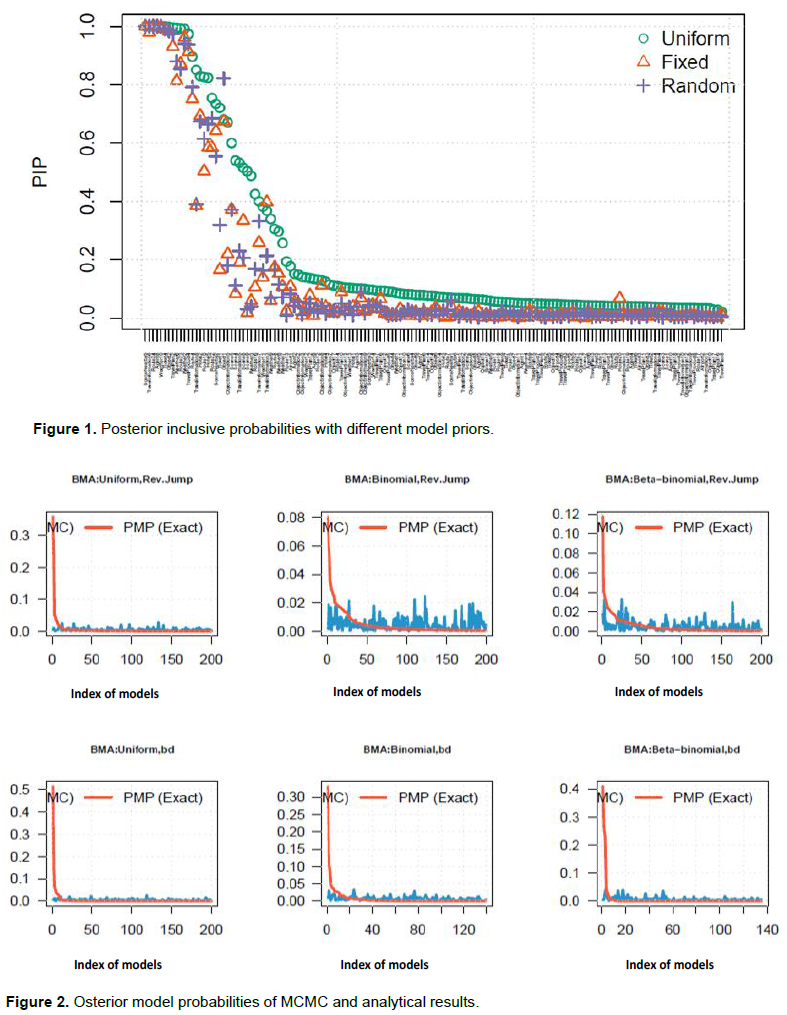
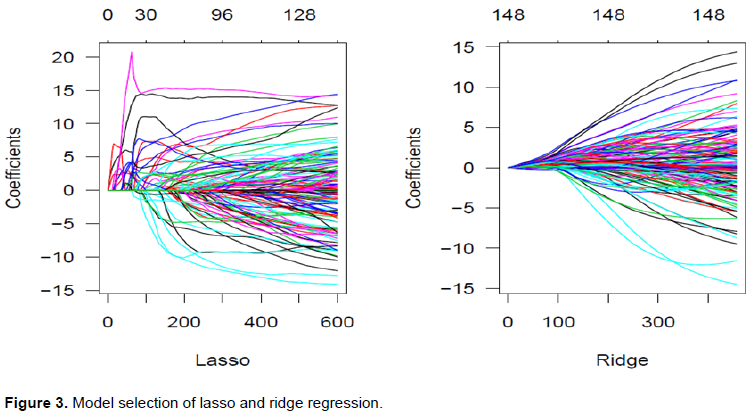
In Figure 1, “uniform” means the model prior is of the uniform type, “fixed” means that the prior is of the binomial type with expectation of 20, and “random” means that the prior is of beta-binomial type. We can see that the model with uniform prior shrinkages smoothly and model with binomial prior shows unstable performance when assigning inclusive probabilities to variables. Nevertheless, all the priors make no huge distinction with each other (Figure 2).
The MCMC methods might suffer from some low-quality approximations, and one way to examine them is to compare them with the analytical results, which are those smooth and red lines in Figure 2. We find that the reversible jump MCMC has better quality than birth-death one. In general, the models with Beta-binomial are accompanied with the worst MCMC approximation, and the models with uniform, that is, a non-informative prior, are poorly approximated through MCMC because the uniform prior requires all the models being assigned with equal weights.
Lasso estimates
The algorithm used to implement Lasso is the coordinate descent method. We first select the penalty parameter,

without cross-validation. The number of
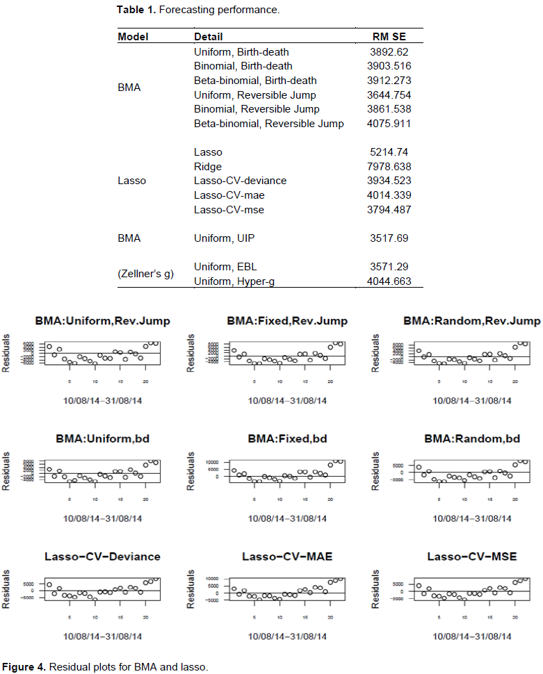
sequence employed is 100. This is the same to ridge regression. Figure 3 explicitly shows the hard-threshoding property of Lasso. In this empirical question, we have 148 independent variables in total. The horizontal axis is the penalty term realization of Equation (10) on the left panel in Figure 3, and the penalty term realization of Equation (11) on the right panel. As we can find, the shrinkage in Lasso is stricter than in Ridge. As the penalty becomes larger, given
, less variables will be screened out in Lasso; while in ridge regression, the shrinkage is milder. Obviously, the chosen model given
might be unstable somehow, therefore when we conduct forecasting we use cross-validation to select proper models, and the criterion of model selection of the cross-validation consists of three types: Deviance, MAE (Mean Absolute Error), and MSE (Mean Squared Error). The results will be discussed in detail in the forecasting performance section.
Forecasting performance
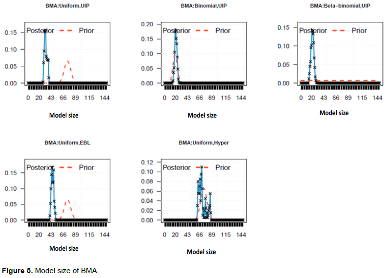
Now we make use of the estimates, and employ the test sample to calculate the RMSE (Rooted Mean of Squared Errors) to make comparison. We use 800 out of 822 observations to estimate and select the model, and let the other 22 to be an out-of-sample for evaluation.
The outcome can be read from Table 1, and the overall distribution of residuals can be seen in Figure 4. It can be read that the best performance is from the BMA with uniform prior and the reversible jump MCMC method. In general, we find that the forecasts using uniform priors are the best, using binomial ranks second and beta-binomial performs worst among the BMA forecasts. This might be an evidence that the non-informative priors actually are good at forecasting. For the lasso, the forecast with MSE cross-validation performs best, and this might be due to that the criterion we use for out-of-sample evaluation is RMSE, which is the closest criterion to MSE. From the numerical results, we do not find whether BMA outperform Lasso, or the other way around in general. If we further look at Figure 4, we also find that the residual sequences have similar patterns, that is, some fluctuations or seasonal patterns on a weekly basis. This implies that the models can be improved considering more complex time series variants such as ARIMA, ARCH, etc. However, in this paper, the linear model is sufficient for comparison of query selections so we will not complicate the settings.
Till now, we only take various model priors and MCMC methods into account. As a crucial element, the Zellner's
seems to play more important roles in forecasting and model selection. We choose three types of
s in our research: fixed with
, the Empirical Bayes, Local type (Hansen and Yu (2001)), and the hyper-

type (Liang et al., 2008).
Based on the “best” model, that is, model with prior uniform and with reversible jump sampler, we conduct the evaluation 5 times, and take the average. The RMSE are 3517.69, 3571.29 and 4044.66, respectively. It can be read that, still, the simple rule wins, since the model with uniform model prior and fixed
has the best performance. It outperforms Lasso, but we cannot say BMA is definitely better than Lasso, since the performance difference is not huge. Nevertheless, the performance reached by both BMA and Lasso is satisfying, compared to the previous results, even though there is space to improve (Figure 4).
Model size and variable selection
First of all, the variable selection here is somewhat confusing in BMA context, since the philosophy of model averaging is proposed against model selection. However, we can treat the posterior inclusion probability (PIP) as the measure of likelihood that certain variables should be included or not. The PIPs demonstrate the posterior probabilities that a variable is included in the models. This is calculated through the summation of the posterior probability of those best models including this variable.
It would be trivial to compare the variable selection if the model sizes are not taken into consideration. In other words, the larger model has more variables, and it has high probability to contain all the variables selected by the small model. Therefore, we first compare the model sizes across different models.
For the BMA models, the model priors affect the model sizes, however, since the likelihoods dominate the posterior as sample size becomes larger, the model sizes are mainly affected by the information underlying the data. In Figure 5, we compare the models with different model priors and Zellner's
s. For the Uniform prior, the expected model size is around 70, while the posterior size is around 30. For the Binomial prior, since we set the expected model size as 20, the posterior is also around 20. For the Beta-binomial, the prior is totally flat over the horizontal axis, while the posterior is still around 20. Zellner's
does affect the posterior model sizes, and we find that more complex
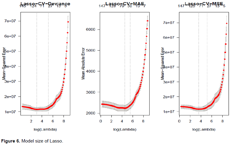
yields more complex posterior size distributions. In addition, all the models with uniform priors has larger model sizes because the prior “drags” the posterior toward it (Figure 5). The model sizes of Lasso with cross-validation, as in Figure 6, are around 30 or slightly above. Cross-validation with deviance selects the best model with the size around 30, similar to the mae type. However, the MSE type are slightly larger.
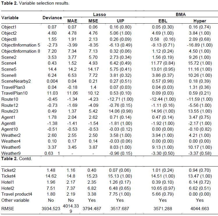
All the comparisons earlier mentioned show that the model sizes differ little between Lasso and BMA. This implies that the intrinsic model size supported by the data is around 30 to have a better forecasting performance. Therefore, it is interesting to see whether Lasso and BMA select similar variables or not. If they select several common variables, the practitioners can then pay more attention to those common queries.
The variable selection results are given in Table 2, and the variables on the list are selected by the Lasso with deviance. If other methods have extra selected variables, then we currently do not report them in the table, since those variables are not important in magnitude, and this does not affect our results because we can see that the estimates of those on-the-list variables are similar. For the BMA estimates, we not only show the parameter estimates, but also give the posterior inclusive probabilities, which is an indicator whether certain variables are not important from BMA point of view. Of course, all the candidate variables has been assigned a PIP, but most of them are very low (Figure 6).