The aim of the present study is to test ESA’s Sentinel-2 (S2) satellites (S2A and S2B) for an efficient quantification of land cover (LC) and forest compositions in a tropical environment southwest of Mount Kenya. Furthermore, outcome of the research is used to validate ESA’s S2 prototype LC 20 m map of Africa that was produced in 2016. A decision tree that is based on significant altitudinal ranges was used to discriminate four natural tree compositions that occur within the investigation area. In addition, the classification process was supported by Google Earth images, and land use (LU) data that were provided by the local Kenyan Forest Service (KFS). Final classification products include four LC classes and five subclasses of forest (four natural forest subclasses plus one non-natural forest class). Results of the Jeffries-Matusita (JM) distance test show significant differences in spectral separability between all classes. Furthermore, the study identifies spectral signatures and significant wavelengths for a classification of all LC classes and forest subclasses where wavelengths of SWIR and the red-edge domain show highest importance for the discrimination of tree compositions. Finally, considerable differences can be seen between the utilized multi-temporal classification set (total of 39 bands from three acquisition dates) and ESA’s S2 prototype LC 20 m map of Africa 2016. A visual comparison of ESA’s prototype map within the investigation area indicates an overrepresentation of tree cover areas (as confirmed in previous studies) and also an underrepresentation of water.
Forests are subject to several policies of individual states and important agreements from the United Nations (UN) (FAO, 2017; IPCC, 2003; UN, 1992, 1997, 2015). The amount of people that directly profit from forests as a natural resource is vast (FAO, 2016b). This also applies to the forests of Mount Kenya National Park, Lewa Wildlife Conservancy, and Ngare Ndare Reserve of the greater Mount Kenya ecoregion. Altogether, these forests shape an extensive ecosystem that represents habitat to numerous endemic species and provide water and other
natural resources to people that live in the mountains and the adjacent foothills (Kenya Wildlife Service, 2010; Winiger and Brunner, 1986). Nevertheless, forests in general and also in Kenya are under massive pressure and in competition with other land-use (LU) systems to this day (McDowell et al., 2020; Barlow et al., 2016; Kenya Forest Service, 2010). Tropical forests are among the most threatened forests and often exposed to radical LU changes and impacts of climate change (Bastin et al., 2019; FAO, 2016a; Lambin et al., 2001). Agriculture is the primary economic activity in the bordering areas of the investigated forest reserve. The increase of agriculturally used areas is a major challenge for sustainable tropical forest management (Kenya Forest Service, 2010). In addition, wildfires, intensified by the effects of climate change, frequently occur within the reserve (Nyongesa, 2015). It is therefore of major concern to understand the structure of forests, to subsequently investigate their interactions with land-use and land cover (LULC) changes, as well as the effects of climate change to support sustainable management of tropical forest resources.
Satellite remote sensing (SRS) can bring important benefits for monitoring LULC changes regarding disturbances and changes within the forest ecosystem (DeFries et al., 1995; Hansen et al., 2013; Townshend, 1992). Quantifying forest cover changes on a large scale is a major challenge to this day. It requires high temporal and spatial accuracy to detect detailed changes within short time periods (Crowther et al., 2015). At the same time resources are limited and researchers need to find efficient solutions for forest monitoring (Wulder and Coops, 2014). Regional anomalies like persistent cloud cover in tropical environments make the process even more complex and limit the availability of up to date SRS data (Asner, 2001). However, techniques of SRS are continuously developing providing new possibilities for Earth observation.
In 2015, Sentinel-2A (S2A) was successfully launched by the European Space Agency (ESA) as part of the Copernicus program. Sentinel-2B (S2B) successfully followed in 2017. All of the data that is produced by the twin satellites is available for free to the scientific community and beyond. The Sentinel-2 (S2) Copernicus mission orbits the earth every five days using both satellites (S2A and S2B) that are equipped with 13 spectral bands at a bandwidth of the visible and near-infrared (VNIR) as well as the short-wavelength infrared (SWIR). The spatial resolution of the spectral bands ranges from 10 m (bands 2-4, and 8) to 20 m (bands 5-7, 8a, 11, and 12) and 60 m (bands 1, 9, and 10) (Fletcher, 2012). As already stated by other authors, strength of the S2 mission is the combination of systematic global coverage, high revisit frequency, multispectral information, wider field of view, and comparatively good spatial resolution (Sola et al., 2018). This enables researchers to see changes in land cover (LC) and forest cover even at a small scale regarding the spatial and temporal resolution. Consequently, numerous studies with the objectives to test S2 products for their technical possibilities have arisen within the last years (Ganivet and Bloomberg, 2019).
Moreover, the Climate Change Initiative (CCI) of the ESA derived a LC classification prototype map of Africa at 20 m spatial resolution that was based on S2 observation data from December 2015 to December 2016 (Fabrizio et al., 2018). Only few studies have so far tested the potential of S2 to discriminate forest types, tree compositions, and tree species. These include but are not limited to: Immitzer et al. (2016) on the classification of tree species in Central Europe (Germany), Laurin et al. (2016) on forest types, dominant species and functional guilds in West Africa (Ghana), Puletti et al. (2017) on forest categories and types in Southern Europe (Italy), Karasiak et al. (2017) on tree species in Southern Europe (France), Persson, Lindberg and Reese (2018) on tree species in Northern Europe (Sweden), and Grabska et al. (2019) on forest types and tree species in Eastern Europe (Poland). However, most of the studies were conducted within a temperate environment. Consequently, more applied research within the tropical environment is needed. Driven by the motivation of the Karantina University and the Kenya Forest Service (KFS), this study aims to fill this research gap through combined use of LU data, Google Earth images, topographic data as well as historic field-based data to develop an efficient method for the creation of spectral signatures. Furthermore, the outcome of the present study will be used for a visual comparison with the existing LC product of ESA’s S2 prototype LC 20m map of Africa 2016. The main objectives of the study are:
i) Testing opportunities and challenges offered by S2 imagery for classification of tropical forest subclasses based on historical field acquisition and terrain information derived from Digital Elevation Models (DEM); ii) Visual comparison of S2 Prototype Land Cover 20 m Map of Africa 2016 and conducted classification within the investigation area;
iii) Creating a detailed classification product for the investigation area that includes LC classes and forest compositions.
Case study area
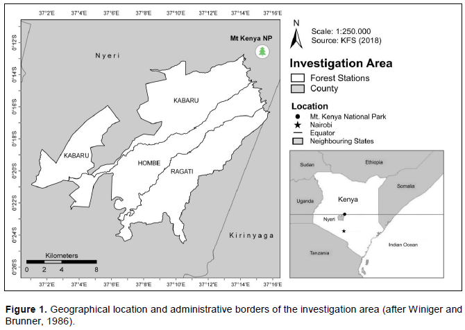
Mount Kenya, also known as Kirinyaga or Kinyaa in the language of Swahili, is the highest mountain massif in Kenya and the second highest in Africa with its highest peak of 5,199 MAMSL. It is located about 150 km north-northeast of the capital Nairobi right on the equator in the center of Kenya (Figure 1).
Part of the greater ecosystem is the Mount Kenya National Park/ Natural Forest in the center and the Lewa Wildlife Conservancy as well as the Ngare Ndare Forest Reserve in the north. Altogether, it shapes an extensive ecosystem that provides habitat to numerous endemic species as well as water to people living in the mountains and the adjacent foothills (Kenya Wildlife Service, 2010). The investigation area is located in the southwest of the Mount Kenya area, bordering the northeastern National Park (Figure 1). Except for a very small part in the east that is attributed to Kirinyaga County, most of the investigation area is part of Nyeri County. Furthermore, it consists of three forest stations: Kabaru, Hombe and Ragati.
Field-based reference data
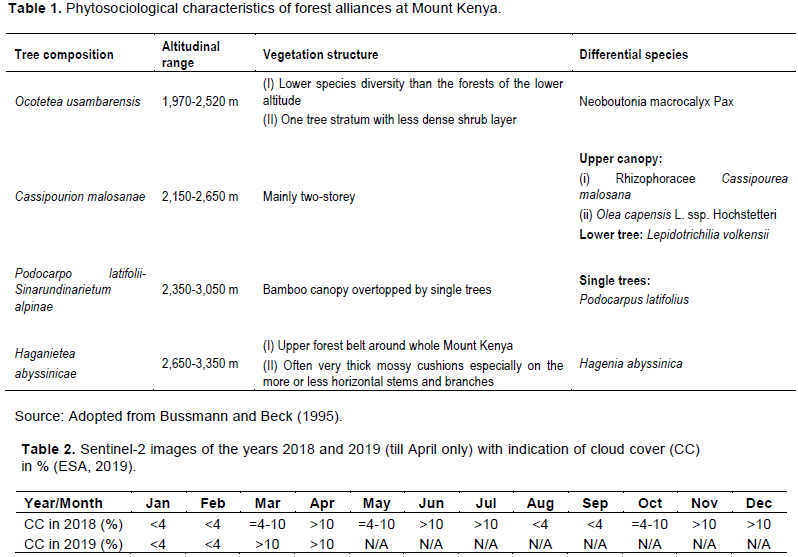
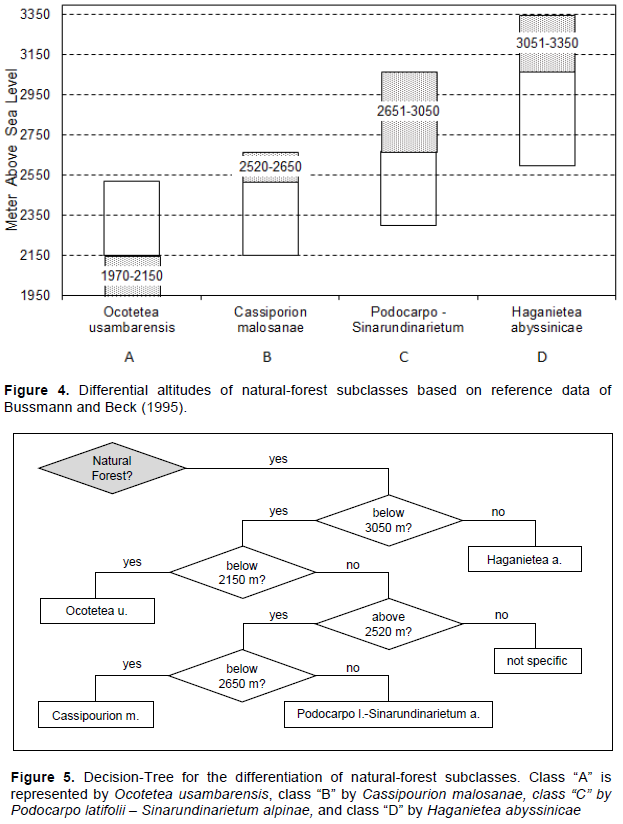
Based on an extensive recording of Mount Kenya’s forests in 1992 to 1994, Bussmann and Beck (1995) accounted 41 tree associations with 47 sub-associations. Furthermore, 10 alliances, 5 orders and 4 classes were identified. Four of the ten alliances can be found in the investigation area southwest of the mountain spreading up to an altitude of 3,400 m (Table 1). Descriptions of the associations give detailed information about the ecological factors, locations, as well as character and differential species. According to Bussmann and Beck (1995), (1) Ocotetea usambarensis is the most common forest formation ranging from 1,970 m to 2,520 m altitude. Differential tree species of this formation is Neoboutonia macrocalyx Pax with a flowering time from September to December (Burrows et al., 2018). Another formation is (2) Cassipourion malosanae which is predominantly two-storey ranging from altitudes of 2,150 m to 2,650 m. Differential tree species of Cassipourion malosanae are Rhizophoracee Cassipoura malosana with a flowering time from September to January and Olea capensis L. ssp. Hochstetteri with irregular flowering intervals of up to seven years (Burrows et al., 2018; Bussmann and Beck, 1995). Third formation is (3) Podocarpo latifolii – Sinarundinarietum alpine at altitudes of 2,350 m to 3,050 m. A bamboo canopy overtopped with single trees of Podocarpus latifolius that in turn represents the differential tree species is characteristic for this forest type. The fourth formation that occurs in the investigation area is (4) Haganietea abyssinicae. At a range of 2,650 m to 3,350 m altitude, this subalpine forest forms the upper forest belt around Mount Kenya. Differential species is H. abyssinicae that is also known as Kosso tree (Bussmann and Beck, 1995).
Digital data applications
Digital data of the research include all data that was used through application of geographic information systems (GIS). Integral part of these data are Sentinel-2 satellite images, the S2 prototype LC 20 m map of Africa 2016, SRTM Digital Elevation Models (DEM), and a LU-map that was provided by the KFS.
Sentinel-2 data
The ESA mission uses twin satellites, equipped with a Multi Spectral Instrument (MSI) including 13 spectral bands at a bandwidth of the visible and near-infrared (VNIR) as well as the short wavelength infrared (SWIR) domain (Table 2) that orbit the Earth every five days. The satellites were launched in 2015 (S2A) and 2017 (S2B). Spatial resolution for the bands of the classical blue (490 nm), green (560 nm), red (665 nm) and near-infrared (842 nm) is 10 m. Four narrow bands in the vegetation red-edge spectral domain (705, 740, 783 and 865 nm) as well as two large SWIR bands (1610 nm and 2190 nm) are at 20 m spatial resolution. Finally, three bands at the spatial resolution of 60 m “[…] are mainly dedicated to atmospheric corrections and cloud screening (443 nm more aerosol retrieval, 945 nm for water vapor retrieval and 1275 nm for cirrus cloud detection)” (Fletcher, 2012: 12).
Sentinel-2 protoptype land covers 20 m of the map of Africa
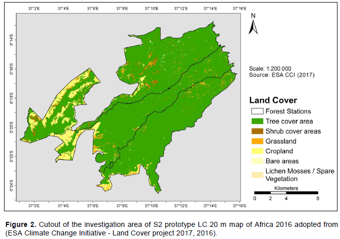
The CCI Land Cover consortium provides global and continental LC maps as result of the CCI Land Cover project. As part of the project, the prototype of a high-resolution LC map at 20 m of Africa was successfully developed (S2 prototype LC 20m map of Africa 2016). Data basis of the map are one year of S2A observations from December 2015 to December 2016. Whereas an official validation of the map has not yet been done, a user evaluation of Lesiv et al. (2017) estimates an overall accuracy of approximately 65% regarding the prototype. The evaluation was done using two independent datasets. Furthermore, the user evaluation highlights an overestimation of individual classes including Tree cover areas (Fabrizio et al., 2018). Figure 2 shows a cutout of the investigation area of the aforementioned S2 prototype LC 20m map of Africa 2016. As can be seen in the map, LC classes that mainly appear within the investigation area are Tree cover areas; Shrub cover areas; Grassland; Cropland; and Bare areas.
The shuttle radar topography mission (SRTM)
SRTM provides digital elevation data of the Earth’s surface between 60° north latitude and 56° south latitude. Spatial resolution of the free available product is close to 30 m, which makes it one of the highest-resolution models of the Earth Data for the SRTM were acquired by the Space Shuttle Endeavour (STS-99) in February 2000 (Farr et al., 2007). The elevation of the investigated area ranges from 1,752 m above sea level in the west to 3,259 m above sea level in the northeast. The elevation model derived from SRTM data was used to determine the height limits (Altitudinal Belts) of the forest type distribution.
Land use map of the kenya forest service
Based on Sentinel and Google Earth data of 2018, a LU map of the forest stations Ragati, Hombe and Kabaru was produced by the Kenya Forest Service (KFS) in 2018. The classification of the map includes Air Strips, Shrublands, Swamps, Tea zone, PELIS, Forest Plantation (including indigenous species as well as Cypress, Pines, and Eucalypts (Mbugua, 2000), Grassland, and Natural Forest Zones that all appear within the investigation area.
Approach
Figure 3 illustrates the overall scheme of the research showing underlying steps of data preprocessing and classification. Before starting with the pre-processing, a status-quo analysis using present LC and LU maps of the investigation area was done. After selecting and downloading satellite products at Level-1C, images had to be pre-processed before starting the classification process. This step of pre-processing involved steps of data correction, data resampling, and calculation of several Vegetation Indices (VIs) that were needed for the classification process at a later stage. Furthermore, image composites of spectral bands and VIs were processed. Representative training samples were created based on the available LU map, and visual interpretation of Google Earth images and tested on their spectral separability using the Jeffries-Matusita (JM) distance test. Finally, a Maximum Likelihood Classification and visual comparison was performed.
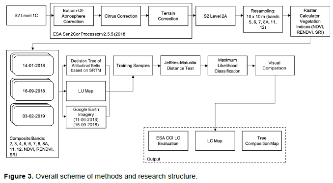
High quality and preferably cloud free imagery are a pre-requisite for further image processing and analysis. Table 1 shows most suitable S2 imagery for the years 2018 and 2019 (until April) via the Copernicus Open Access Hub (OAH) portal of the ESA. Persistent cloud cover is characteristic for the study area, nevertheless a total of six images with a cloud cover less than 4% could be acquired.
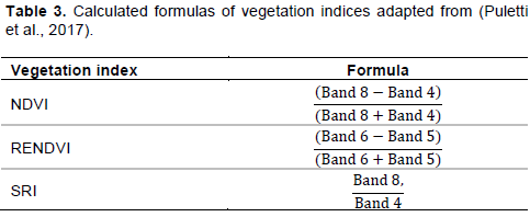
Due to their suitable distribution of cloud cover, three acquisition dates (14th January, 2018, 16th September, 2018 and 3rd of February, 2019) were chosen for further pre-processing including image correction, spatial resampling and the calculation of Vegetation Indices (VIs). The second step of the overall process and first partial step of the image pre-processing was an upgrade of Level-1C images to Level-2C. This was performed with the support of ESA’s Sen2Cor Processor v2.5.5 (ESA, 2018). The process of the upgrade for all three images included atmospheric correction, cirrus correction, and terrain correction, respectively. The spectral bands of S2 satellite images come with different spatial resolutions ranging from 10 m to 60 m. To get a suitable overall resolution for canopy applications as well as in order to exploit the potential of the visible R, G, B and the NIR bands at 10 m, all 20-m bands were resampled to a spatial resolution of 10 m (Puletti et al., 2017). The process was performed, using the nearest neighbor function of the Resampling tool in ArcGIS 10.7 which is primarily used for discrete data, such as LC classifications, since it does not change the digital values of the pixels (Patil et al., 2012). Bands at a spatial resolution of 60 m were not used for further processing since they are mainly designed for atmospheric corrections (Fletcher, 2012). After resampling all bands from a resolution of 20 m to a resolution of 10 m, resampled spectral bands as well as original bands with a resolution of 10 m were used to calculate several VIs (Table 2).
The last step of data pre-processing involved the creation of the following five image composites using the resampled bands (2, 3, 4, 5, 6, 7, 8, 8A, 11, 12) as well as the computed VIs (NDVI, RENDVI, SRI):
(i) Band 2, 3, 4, 5, 6, 7, 8, 8A, 11, 12
(ii) Band 2, 3, 4, 5, 6, 7, 8, 8A, 11, 12, NDVI
(iii) Band 2, 3, 4, 5, 6, 7, 8, 8A, 11, 12, RENDVI
(iv) Band 2, 3, 4, 5, 6, 7, 8, 8A, 11, 12, SRI
(v) Band 2, 3, 4, 5, 6, 7, 8, 8A, 11, 12, NDVI, RENDVI, SRI.
At the same time, cloud cover within the image composites was removed to prevent interferences during the classification process. The first step of the classification process was the determination of natural-forest subclasses using the reference data of Bussmann and Beck (1995). Unique altitudinal belts regarding the occurrence of different tree alliances were derived from the reference data. The altitudinal belts for indigenous forest are from 1,970 to 2,150 m altitude for Ocotetea usambarensis, 2,520 m to 2,650 m altitude for Cassipourion malosanae, 2,651 to 3,050 m altitude for Podocarpo latifolii - Sinarundinarietum alpinae, and 3,051 m to 3,350 m altitude for Haganietea abyssinicae (Figure 4). The derived decision tree for the four different subclasses of Natural Forest is shown in Figure 5.
With reference to the decision tree, class “A” is represented by Ocotetea usambarensis, class “B” by C. malosanae, class “C” by Podocarpo latifolii – Sinarundinarietum alpinae, and class “D” by Haganietea abyssinicae. The decision tree starts with a general query whether a pixel is defined as Natural Forest (four subclasses) or non-natural forest (Forest Plantation). This decision can be determined by the LU-map described by KFS. If the forest is declared as Natural Forest, the next question is whether a pixel is above or below an altitude of 3,050 m. If the pixel of Natural Forest is above 3,050 m altitude, it is declared as class “D”. If not, the next question is whether the Natural Forest is above or below 2,150 m altitude. Below 2,150 m altitude and different from class “D”, Natural Forest is defined as class “A”. Above 2,150 m altitude, the next question is whether the pixel is above or below 2,520 m altitude. If the pixel is below 2,520 m altitude, it is not possible to define the Natural Forest as a specific class. These pixels cannot be used within training sample since they are located in a transition zone of two or more forest subclasses. If the pixel is above 2,520 m altitude, the next question is whether it is above or below 2,650 m altitude. If it is above 2,650 m altitude and different from class “D”, it is defined as class “C”. If it is below 2,650 m altitude and different from class “A” and class “C”, it is defined as class “B”. Finally, information of the four subclasses of Natural Forest with reference to their unique altitudinal appearance was used to create four shapefiles of the areas that are potentially covered by the same classes. In addition, shape files of all subclasses were collated to the LU class of Natural Forest and intersected if not coextensive to each other.
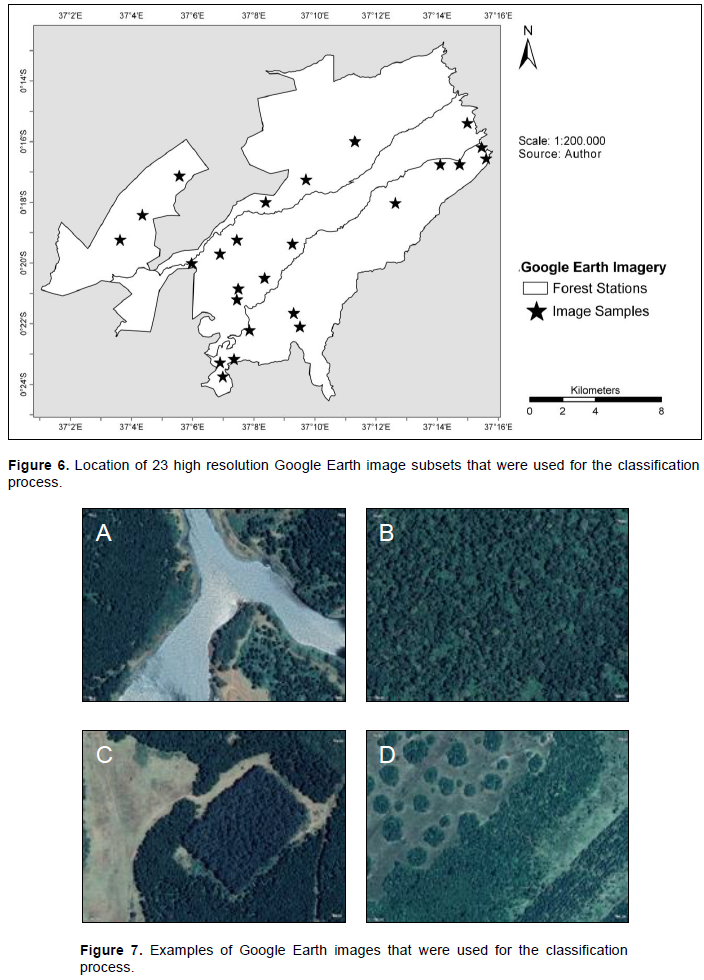
The third step within the classification process involved the selection of training samples for all classes. For this purpose, 23 high resolution satellite image subsets (1 m spatial resolution) from Google Earth were imported into ArcGIS 10.7. The locations of the individual images can be seen in Figure 6. The acquisition date of the image subsets (Image Copyright 2019 CNES / Airbus) was June 6th, 2018 and September 16th, 2018 which partially coincide with the acquisition date of the second S2 image used within the study.
Figure 7 shows four examples of image subsets that were used for the classification process. (A) Classes of Water and Forest Plantation. (B) Natural-forest subclass of Ocotetea usambarensis. (C) Classes of Grassland and Forest Plantation (D) Class of Grassland and the natural-forest subclass of Ocotetea usambarensis (Google, 2019).
Based on the decision tree (Figure 5), Google Earth images (Figure 7), and the LU map by the KFS multiple training samples for a total of nine LC classes were defined, using the Training Sample Manager in ArcGIS Pro 2.2.4 (ESRI, 2019). As can be seen in Table 3, a total amount of 9067 pixels are separated into the classes of Water (585), Bare Land (941), Forest Plantation (2702), Tea (154), Ocotetea usambarensis (1629), Podocarpo latifolii – Sinarundinarietum alpinae (982), H. abyssinicae (136), C. malosanae (1377), and Grassland (561).
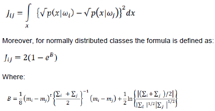
To analyze the quality of training samples of LC classes and forest subclasses, spectral distances were calculated for all classes by using the JM distance test. The test measures the average distance between two spectral class density functions and is defined by Wacker and Landgrebe (1972) as:
Where mi is the first spectral signature vector, mj is the second spectral signature vector, Σi is the covariance matrix of mi, and Σj is the covariance matrix of mj. Results of the test close to 0 imply identical signatures whether values close to 2 imply completely different signatures (Richards and Jia, 2006). Spectral distances were computed for all three days using band composites of 10 bands (2, 3, 4, 5, 6, 7, 8, 8A, 11, 12), 10 bands (similar to step one) plus NDVI, 10 bands (similar to step one) plus RENDVI, 10 bands (similar to step one) plus SRI, and 10 bands (similar to step one) plus NDVI, RENDVI, and SRI for each day.
The next step of the classification process was the performance of a Maximum Likelihood Classification. For this purpose, all training samples (Table 3) were used to produce classified satellite images for each acquisition date. In addition, a multi-temporal classification combining all three products was computed. Based on the results of spectral separability, the following layer stacks were used for Maximum Likelihood Classifications:
(1) 14-01-2018 (band 2, 3, 4, 5, 6, 7, 8, 8A, 11, 12, NDVI, RENDVI,
SRI)
(2) 16-09-2018 (band 2, 3, 4, 5, 6, 7, 8, 8A, 11, 12, NDVI, RENDVI,
SRI).
(3) 03-02-2019 (band 2, 3, 4, 5, 6, 7, 8, 8A, 11, 12, NDVI, RENDVI, SRI).
(4) Multi-temporal (14-01-2018 + 16-09-2018 + 03-02-2019).
SRI).
(3) 03-02-2019 (band 2, 3, 4, 5, 6, 7, 8, 8A, 11, 12, NDVI, RENDVI, SRI).
(4) Multi-temporal (14-01-2018 + 16-09-2018 + 03-02-2019).
Spectral distances
Table 4 shows the calculated spectral distances between all tree subclasses that include Ocotetea usambarensis, C. malosanae, Podocarpo latifolii – Sinarundinarietum alpinae, Hagenietum abyssinicae, and Forest Plantation for the band composite of 10 bands and three Vis. Most class pairs show equal separability values for the three different dates, but some considerable differences are apparent. The lowest overall value is shown for the class pair C. malosanae versus Ocotetea usambarensis on September 16th, 2018 with a spectral distance of 1.65 (JM). In contrast, all other comparisons show excellent values at the same day. Similar values can be seen on February 3rd, 2019 where spectral distance between C. malosanae versus Ocotetea usambarensis is slightly higher (1.81 [JM]) but still below 1.9 (JM). In addition, a difference between the two aforementioned dates is shown for the class pair Haganietea abyssinicae versus C. malosanae. On September 16th, 2018, the comparison shows an excellent value of 2.00 (JM). On February 3rd, 2019, the comparison shows a good value of 1.90 (JM). Best overall values are identified on January 14th, 2018 with a lowest value of 1.90 (JM) for the class pair Ocotetea usambarensis versus Forest Plantation. However, all other spectral distances of January 14th are above 1.90 (JM), which makes it a good day for separation of all the Natural Forest subclasses and the Forest Plantation class.
Spectral signatures
Spectral signatures and profiles were computed for all three S2 acquisition dates. Furthermore, class reflection characteristics were analyzed using box plot statistics of all bands and VIs for each date. In the following, the spectral signatures of one acquisition date (January 14th, 2018) are described.
Figure 8 shows a spectral profile of mean reflection values on January 14th, 2018. The graph shows that all classes except from Grassland show highest amplitudes between band 5 and band 11 with the highest point at band 8A. Grassland shows the highest amplitude at band 11. Band 8 and band 8A seem most feasible for the differentiation of LC classes since mean value lines of the classes are further apart in comparison to other bands. With reference to the mean reflection of all classes, values of Water stand out in almost all spectral bands (Figure 8). Mean values for water are by far the lowest compared to all other classes. For all non-water classes (mostly vegetated except from Bare Land) the significance of red-edge is apparent. This is especially shown comparing the class Tea to classes of Grassland and Bare Land where mean values at bands 6 (3035.8 and 2155.01/2291.89), 7 (3699.98 and 2442.22/2680.53), and 8 (3965.68 and 2629.5/2803.66) differ considerably. Values of Grassland (2629.5) and Bare Land (2803.66) are similar in the NIR spectrum (band 8) with highest differences in the SWIR at Band 11 (3007.94/1971.43) and 12 (2100.06/1154.84). Clear differences can be seen in all three VIs (NDVI, RENDVI, SRI) for Water (0.3/0.15/1.27), Grassland (0.47/0.22/2.29), Tea (0.8/ [0.44]/11.95), and Bare Land (0.68/ [0.4]/0.55). Only RENDVI shows similar values when comparing the class of Tea (0.44) and with the class Bare Land (0.4).
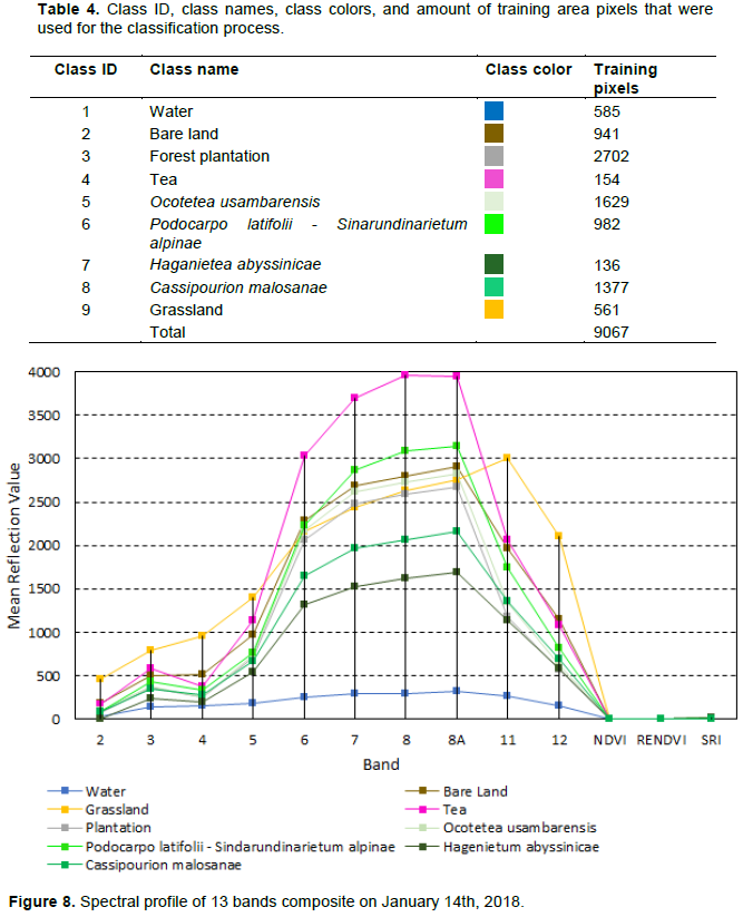
Although, mean reflection values of all forest subclasses (Figure 8) are lot denser compared to those of non-forest classes, major differences appear within the red-edge region. Lowest difference of mean values is measured between Ocotetea usambarensis and Forest Plantation. For all red-edge bands, the difference between these two classes is below 160 reflection units. On the contrary, highest separability can be determined between Podocarpo latifolii - Sinarundinarietum alpinae and Haganietea abyssinicae with up to nearly 1500 reflection units in the NIR (band 8) and red-edge (band 8A). Red-edge values of Grassland and Bare Land are quite close to the values of Ocotetea usambarensis and Forest Plantation. Considering the VIs, some forest subclasses show same values. This accounts for Ocotetea usambarensis (0.82) and Forest Plantation (0.82) at the NDVI, Ocotetea usambarensis (4.9), Podocarpo latifolii - Sinarundinarietum alpinae (4.9), and Forest Plantation (4.9) at the RENDVI, as well as C. malosanae (0.42) and Haganietea abyssinicae (0.42) at the RENDVI.
A detailed visualization of all ten spectral bands on 14 January, 2018 is shown in Figure 9. Figure 10 shows band reflection statistics of the three VIs. With reference to Grassland, it is possible to discriminate the class from all others within bands 2, 3, 4, 5, 11, 12, and the NDVI. At bands 6, 7, 8, 8A and the RENDVI as well as the SRI, the interquartile range of Grassland overlaps completely or partially with other classes. Almost the same applies for the class of Bare Land. The only difference in comparison to Grassland is that the interquartile range overlaps with Haganietea abyssinicae at the NDVI. Furthermore, Tea can be discriminated from other classes at bands 3, 5, 6, 7, 8, and 8A. At all other bands as well as the VIs, the interquartile range of Tea overlaps with the interquartile range of other classes. The Water class can be separated at almost every spectral band and VI. Only exception is given by the RENDVI where the interquartile range of Water overlaps with Grassland. Consequently, all four non-forest classes can be separated quite well on January 14th, 2018.
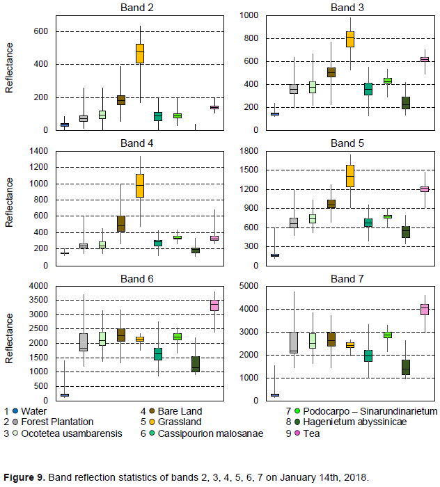
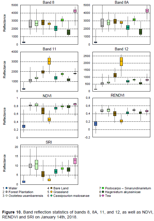
A discrimination of forest subclasses is much more complex which is also confirmed by the results of spectral distances. Probably the clearest discrimination of forest subclasses is identified for Haganietea abyssinicae. Especially at bands 2 and 3 the difference of Haganietea abyssinicae to all other classes is very high. At bands 4, 5, 6, 7, 8, and 8A the interquartile range overlaps with other classes to a very small extent. Furthermore, a total overlap with other classes is seen at bands 11, 12 and at all VIs. For the forest subclass Podocarpo latifolii – Sinarundinarietum alpinae most effective discrimination can be seen at bands 3, 8, and 8A where the interquartile range overlaps just slightly with other classes. According to the box plots of bands 6, 7, 8, and 8A, C. malosanae can be differentiated best in the spectral region of red-edge and NIR. The forest subclasses of Ocotetea usambarensis and Forest Plantation and most difficult to separate. Except for band 11, the interquartile range of both classes overlaps within all other bands. This result is congruent with results of spectral distances, where comparisons between Ocotetea usambarensis and Forest Plantation show the lowest values on January 14th, 2018.
Land cover classification
Table 5 lists area statistics of all LC classes on January 14th, 2018, September 16th, 2018, and February 3rd, 2019 combined to a multi-temporal composite. The composite classification map (Figure 11) is illustrated below. Forest subclasses cover a total area of 189 km2 (76%), whereas non-forest classes cover an area of 60 km2 (24%).
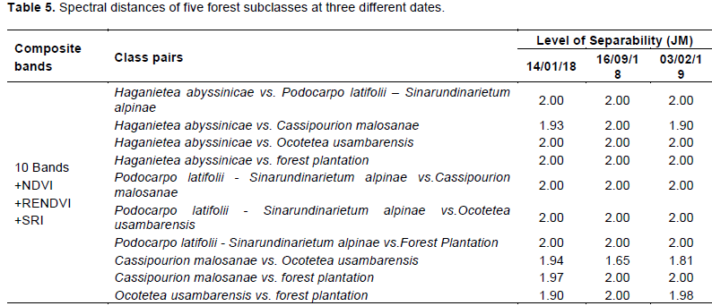
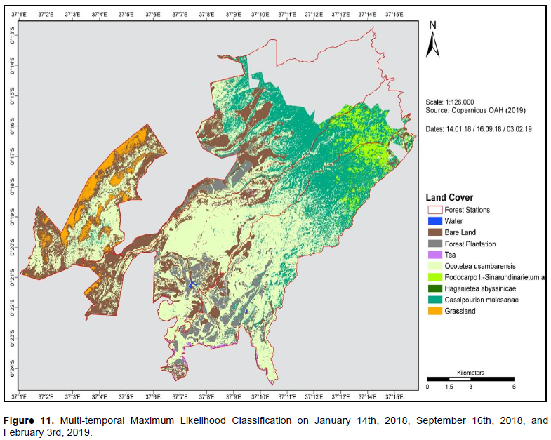
Figure 11 shows several spatial characteristics of the nine LC classes for multiple dates that for the most part coincide with characteristics of single-dates. (1) Small water bodies are visible east and west of the southern center, similar to all other dates. (2) Bare Land is located in the western and central areas of the investigation area including small expansions in the northeastern parts. (3) Forest Plantation covers large parts of southern central areas with further coherent areas in the central north (similar to all other dates). (4) Small areas of Tea are visible in the southern investigation area. (5) Ocotetea usambarensis covers large parts of the southern center, representing the largest class with an extent of more than 40%. (6) Podocarpo latifolii - Sinarundinarietum alpinae is visible in high altitudes in the northeast (similar to all other dates). (7) Small areas of Haganietea abyssinicae appear within the highest altitudes in the northeast. (8) C. malosanae covers large parts of the central east and north with some additional coveage in the west and (9) Grassland covers the western edge of the investigation area.
Visual comparison
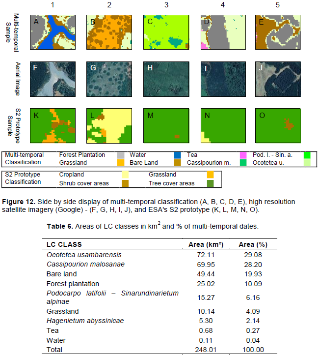
Figure 12 shows a side by side display of multi-temporal classification, Google imagery and ESA's S2 prototype samples. Furthermore, Table 6 shows a legend of Figure 12 including class names as well as class colors of visible LC classes within the samples.
Image subset “F” in row 1 shows a significant water body surrounded by different LC. This can be verified by the multi-temporal sample “A” of row 1 that clearly shows the class of Water, Bare Land, Forest Plantation, Ocotetea usambarensis, and some individual pixels of C. malosanae, and Tea. On the contrary, no water is determined at sample “K” of row 1 of the S2 prototype. Instead, areas of Shrub cover areas and Grassland are surrounded by Tree cover areas. Image subset “G” of row 2 shows sparsely vegetated areas with several small islands of trees and shrubs surrounded by areas of trees and shrubs. This is partially verified by multitemporal sample “B” of row 2 that shows several small islands of Bare Land surrounded by Grassland, and Ocotetea usambarensis. In addition, individual pixels of C. malosanae appear. Sample “L” of ESA’s S2 prototype shows a large area of Cropland surrounded by Tree cover areas and small areas of Shrub cover areas and Grassland. No islands can be identified within the sample of ESA’s S2 prototype. At first glance, Google Earth image “H” of row 3 shows different forest types. This is confirmed by the multi-temporal sample “C” of row 3 that shows forest subclasses of C. malosanae, P. latifolii – S. alpinae, and Ocotetea usambarensis as well as a small area of Bare Land on the bottom right. Sample “N” of row 3 of ESA’s S2 prototype exclusively shows Tree cover areas with a small number of Shrub cover areas. Image subset “I” of row 4 shows two different types of forests with fields of tea in the bottom left. In addition, several paths/streets cross the image. This is mainly verified by multi-temporal sample “D” of row 4 that shows classes of Forest Plantation, O. usambarensis, C. malosanae, and Tea. Moreover, aforementioned paths/streets are represented by small areas of Bare Land within the classified image. Sample “N” of row 4 of ESA’s S2 prototype shows mostly Tree cover areas with a small area of Cropland in the bottom left. Finally, image subset “J” of row 5 shows non-vegetated areas separated by large areas of tree cover that indicate human impact. Multi-temporal sample “E” of row 5 is partially correspondent to this. The classification is characterized by large areas of Forest Plantation and Bare Land but includes a differentiation between Forest Plantation and Ocotetea usambarensis as well as some pixels of Tea. Hence, a differentiation of trees is shown in the multi-temporal classification but not in the Google Earth image. Sample “O” of ESA’s S2 prototype shows predominantly Tree covered areas with an individual spot of Shrub. In conclusion, the most significant difference between the multi-temporal classification and ESA’s S2 prototype is the appearance of water (row 1), the differentiation of details within the LC (row 1 to 5), and the discrimination of forest subclasses (row 1, 3, 4, and 5). Moreover, the overrepresentation of Cropland as well as Tree cover areas (Figures 2 and 11) can be confirmed as stated by Fabrizio et al. (2018).