ABSTRACT
Stochastic models have proven to be practically fundamental in fields such as science, economics, and business, among others. In Malawi, stochastic models have been used in fisheries to forecast fish catches. Nevertheless, forecasting water levels in major lakes and rivers in Malawi has been given little attention despite the availability of ample historical data. Although previous multichannel seismic surveys revealed the presence of low stands (sediment bypass zone) in Lake Malawi indicating that since the beginning of its formation, important water level fluctuations have been occurring, these previous surveys failed to predict and highlight much more clearly the status of these levels in the future. Therefore, the main objective of the study was to fill these research gaps. The study used Autoregressive (AR), Moving Average (MA), Autoregressive Moving Average (ARMA) and Autoregressive Integrated Moving Average (ARIMA) processes to select the appropriate stochastic model. Based on lowest Normalized Bayesian Information Criterion (NBIC), Root Mean Square Error (RMSE), Mean Absolute Percentage Error (MAPE), Mean Forecast Error (MFE), Maximum Absolute Percentage Error (MAXAPE), Maximum Absolute Error (MAXAE), and Mean Absolute Error (MAE) - ARIMA (0,1,1) model is found suitable for forecasting Lake Malawi water levels which shows negative trend up to 2035. The study further predicted that Lake Malawi water levels will decrease from the current average level of 472.97 m to an average of 468.63 m for the next 18 years (up to 2035).
Key words: Forecasting, Lake Malawi, modelling, stochastic, time series, water levels.
Time series stochastic process is a set of random variables where the index t takes values in a certain set C (Alonso and Garcia-Martos, 2012). The process provides attractive modeling techniques for forecasting and planning because historical data can be used to a reasonable level of certainty (Box et al., 2015). The model deals with a sequential set of data points, measured typically over successive times. It is mathematically defined as a set of vectors where t represents the time elapsed (Hipel and McLeod, 1994). The variable x(t) is treated as a random variable and the measurements taken during an event in a time series are arranged in a proper chronological order. The principles of stochastic process are to describe and summarize time series data, fit low-dimensional models and make forecast (Box et al., 2015). Time series data have many forms and represent different stochastic processes. According to literature, Autoregressive (AR) and Moving Average (MA) models have been widely and commonly used in different fields (Box and Jenkins, 1970; Hipel and McLeod, 1994). The combination of AR and MA models forms Autoregressive Moving Average (ARMA). However, ARMA model only works with stationary time series data. Thus, from application viewpoint, ARMA models are inadequate to properly describe non-stationary time series, frequently encountered in practice. For this reason, the Autoregressive Integrated Moving Average (ARIMA) model (Box and Jenkins, 1970) is proposed. The ARIMA model is a generalisation of an ARMA model which includes the case of non-stationarity as well (Chang et al., 2012). The model was first proposed by Box and Jenkins in the early 1970s and was often termed as Box-Jenkins models (Stuffer and Dhumway, 2010). Because ARIMA model is relatively systematic, flexible and can grasp more original time series information, it is widely used in meteorology, engineering technology, marine, economic statistics, prediction technology, hydrology and water resources studies (Yevjevich, 1972; Aksoy et al., 2013; Cryer and Chan, 2008; Kantz and Schreiber, 2004).
In Malawi, ARIMA model has been commonly used in fisheries to forecast fish catches (Zindi et al., 2016; Lazaro and Jere, 2013; Singini et al., 2012; Mulumpwa et al., 2016). Nevertheless, forecasting water levels in major lakes and rivers in Malawi has been given little attention despite the availability of ample historical data. On the same note, although previous multichannel seismic surveys (Scholz and Rozendahl, 1988; Johnson and Davis, 1989; De Vas, 1994) revealed the presence of low stands in Lake Malawi indicating that since the beginning of its formation, important water level fluctuations have been occurring, these previous surveys failed to predict and highlight much more clearly the status of these levels in the future. Consequently, the present study was designed to fill these research gaps.
Study area and physiography
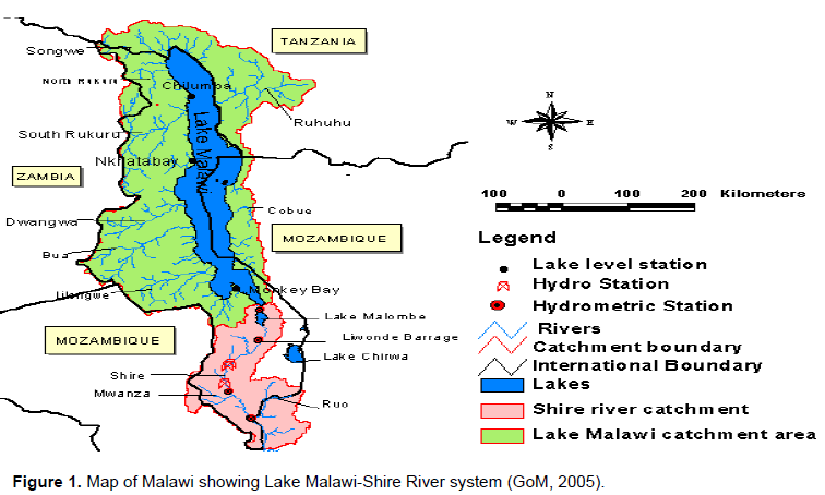
The study was conducted in Lake Malawi, located at the southern end of the Great Rift Valley region. It is an elongated lake surrounded by mountains with highest elevations to the north. Figure 1 shows that the boundaries of Lake Malawi cross Mozambique and Tanzania with an outlet in the southern end. The lake is ranked as the ninth largest and third deepest freshwater lake in the world with an estimated total area of 28,750 km2 and a volume of about 7725 km3. The Shire River is the outlet of Lake Malawi and flows approximately 410 km from Mangochi to Ziu Ziu in Mozambique, where it drains into Zambezi River (Shela, 2000). According to Shela (2000), the physiography of upper Shire has offered opportunities for regulating river flows and subsequently lake levels, with possible expansion. The middle section of Shire River is estimated to be 80 km and is very steep characterised by rock bars and outcrops with water falls of about 370 m.
Data collection and time series model description
Lake Malawi has been there over the years. Literature has shown that in early 1924, Dixey attempted to understand the hydrology of Lake Malawi (Dixey, 1924). However, he failed due to lack of hydrological data (Dixey, 1924). Later in the years, the fear of period of no outflow by authorities greatly forced them to seriously monitor the Lake levels (Drayton, 1984). Department of Water Resources seriously embarked on collection of water levels data later in the years; however, the data collected from 1950s to somewhere around 1980s were too complex and the quality was too inconsistent. Similar observation was reported by Kaunda (2015). Because of these past data anomalies, the present study analysed the univariate time series data of Lake Malawi water levels from 1985 to 2016 period. Figure 1 shows that the Department of Water Resources collects water levels data from three stations along the lake shore (Chilumba, Nkhatabay and Monkey Bay). The water level is normally the average of three records ignoring the water level gradient which is between the north and south tip of the lake (Kumambala, 2010).
Application of stochastic models
The study used two linear time series models known as Autoregressive (AR) (Box and Jenkins, 1970) and Moving Average (MA) (Zhang, 2003) models. These models were combined to form Autoregressive Moving Average (ARMA) (Cochrane, 1997). The combination of these two models were based on famous Box-Jenkins principle (Box and Jenkins, 1970) also known as the Box-Jenkins models.
Autoregressive Moving Average (ARMA) Model
An ARMA (p,q) model which is a combination of AR(p) and MA (q) models was developed. In an AR (p) model, the future value of a variable was assumed to be a linear combination of (p) past observations and a random error together with a constant term. Mathematically, the AR (p) model (Hipel and McLeod, 1994) is expressed as
where and are the actual value and random error at time period t, respectively, (i=1, 2 ... p) are model parameters and c is a constant. Just as an AR (p) model regress against past values of the series, an MA (q) model uses past errors as the explanatory variables. The MA (q) is given by (Hipel and McLeod, 1994) and is expressed as:
All inferential and descriptive statistics were performed using International Business Management Statistical Package for Social Scientists software (IBM SPSS 20) (IBM Corp, 2011).
Model selection
The stationarity of a stochastic process was visualized in form of a data plot as shown in Figure 2. According to Hipel and McLeod (1994), identification of stationarity in time series data is a necessary condition for building a time series model that is useful for forecasting. Sankar (2011) defined time series stationarity as a set of values that vary over time around a constant mean and constant variance.
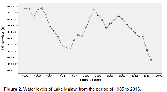
According to Hipel and McLeod (1994), time series data showing seasonal patterns are usually non-stationary in nature. From Figure 2, it is very apparent that the time series data from Lake Malawi water levels is non-stationary due to unstable means which increase and decrease at some points throughout 1985 to 2016. Similar observation was reported by several authors in Lake Malawi (Lazaro and Jere, 2013; Singini et al., 2012; Mulupwa et al., 2016; Zindi et al., 2016). Given these difficulties in Lake Malawi water levels time series data, first order differencing of the data and stationary test were conducted on the newly constructed series of the data. Since the newly constructed data was stationary in mean, the next issue was how to select an appropriate model that can produce accurate forecast based on the description of historical pattern in the data and how to determine the optimal model order. In this case, the values of p and q in the ARIMA model were identified by plotting autocorrelogram and partial autocorrelogram presented in Figure 3.
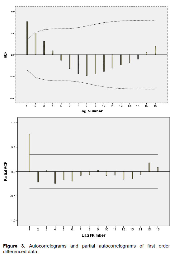
Figure 3 illustrated that autoregressive model of order p(AR (q)) was stationary and moving average model of order q(MA (q)) was good. Guti´errez-Estradade et al. (2004) explained that a good autoregressive model of order p(AR (q)) has to be stationary and a good moving average model of order q(MA (q)) has to be invertible. The invertibility and stationarity gives a constant mean, variance and covariance which is a necessary condition for forecasting (Singini et al., 2012). Following Hipel and McLeod (1994), autocorrelation and partial autocorrelation coefficients (ACF and PACF) of up to 16 lag were considered. The type and order of the adequate model required to fit the series was determined. As the ACF values diminished rapidly with increasing lags, it was assumed that lynx series was stationary. The autocorrelation and partial autocorrelation coefficients (ACF and PACF) of various orders of differenced series of data were computed and presented in Table 1. The basic principle of model parsimony states that the model with smallest number of parameters is to be selected so as to provide an adequate representation of the underlying time series (Chatfield, 1996). In other words, out of a number of suitable models, it is very important to consider the simplest model while still upholding an accurate description of inherent properties of the time series (Zhang, 2007).
As discussed by Hipel and McLeod (1994), a number of ARIMA models were competed in order to select the simplest one as shown in Table 2. Hipel and McLeod (1994) observed that the more complicated the model, the more possibilities will arise for departure from actual model assumptions. In other words, with the increase of model parameters, the risk of model overfitting also subsequently increases. Although over fitted time series models describe the data very well, it may not be suitable for future forecasting. Therefore, genuine attention was given to select the most parsimonious model among all other possibilities. Using the coefficients in Table 1, various ARIMA models were identified and the models together with their corresponding fit statistics are presented in Table 2. The Root Mean Square Error (RMSE) which measured how much dependent series varies from its model-predicted level was lowest (0.28) in ARIMA (1,1,0) model which according to Cao and Francis(2003), indicated a good forecast of the model. Similarly, Mean Absolute Error (MAE) also known as Mean Absolute Deviation was lowest (0.19) in ARIMA (1,1,0) model which indicated a good forecast of the model. In other words, the magnitude of overall error occurring due to forecasting was very small.
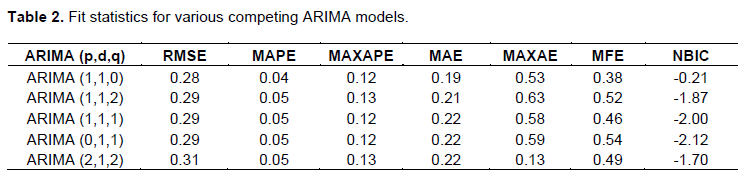
It was further noted that Mean Absolute Percentage Error (MAPE) was lowest and smallest in ARIMA (1,1,0) meaning that the percentage of average absolute error occurring was very small. In other words, the opposite signed errors did not offset each other. It was further interesting to note that Maximum Absolute Percentage Error (MAXAPE) and Maximum Absolute Error (MAXAE) expressed as percentage was very small in ARIMA (1,1,0) model indicating overall good model fit. According to Czerwinski et al. (2007), the best model should have adequate accuracy measures (RMSE, MAE) and lowest Normalised BIC for it to have accurate forecasts. Therefore, ARIMA (1,1,0) model was selected because it had lowest RMSE, MAE, MFE and Normalized Bayesian Information Criterion (NBIC). It was further observed that the coefficients of the parameters of ARIMA (1,1,0) model were significant. According to Czerwinski et al. (2007), the model which indicate lowest normalized BIC and is significant (p<0.05) is a better model in terms of forecasting performance than with large normalized BIC. Estimates of the selected ARIMA (1,1,0) model are presented in Table 3.
Based on the study findings, the most suitable model for forecasting Lake Malawi water levels was confirmed to be ARIMA (1,1,0).
Model systematic checks
The basic model verification is concerned with checking the residues to see if they contain any systematic pattern which could still be eliminated to improve the performance of the selected model. Therefore, the selected ARIMA (1,1,0) model was subjected to autocorrelations and partial autocorrelations of residues of various orders. Various autocorrelations of up to 24 lags were computed and plotted as shown in Figure 4. The results showed that none of the autocorrelation was significantly different from zero at any reasonable level. This implied that the selected ARIMA (1,1,0) model was an appropriate model for forecasting Lake Malawi water levels.
It is very apparent from Figure 4 that autocorrelations of the coefficients are within 95% confidence interval, suggesting that the selected model was well fitted in time series model and had an accurate forecast.
Forecasting
Using the selected ARIMA (1,1,0) model, the forecast of Lake Malawi water levels was made from 1985 to 2035.
For preciseness and accurateness sake, only observations from 2005 to 2016 were compared with the forecasted values as shown in Table 4. Figure 5 on the other hand, indicates the forecasted value from 1985 to 2035. Czerwinski et al. (2007) explained that the forecasted and actual values need to be very close, meaning that the forecasting error must be very low for the model to qualify as good. As observed in Table 4, the noise residues were a combination of positive and negative errors indicating that the model had a good performance of forecasting. It was further interesting to note that the magnitude of the difference between the forecasted and actual values were very low indicating a good forecasting performance. In Figure 5, it is very apparent that Lake Malawi water levels are fluctuating with a negative trend. Such negative trend will continue up to 2035.
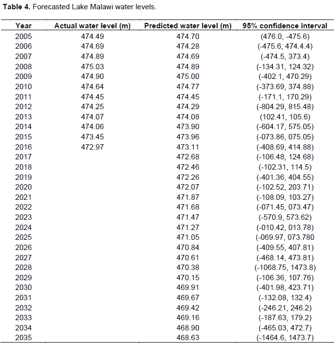
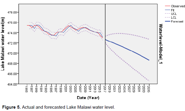
Figure 5 further indicated that values for water levels increased during 2006 to 2010 and decreased up to 2015 when compared to values of 2005. However, the trend declined continuously up to 2035. The basic principle of ARIMA model assumes that time series data is linear and follows a particular known statistical distribution such as normal distribution (Cochrane, 1997). Therefore, it may be concluded that the trend in this study behaved in a manner consistent with ARIMA principle which is assumed to follow a certain probability model described by joint distribution of random variable. It is also interesting to note that time series is non-deterministic in nature such that it cannot predict with certainty what will occur in the future. Based on this observation, the study indicated that there is high probability that Lake Malawi water levels will decrease as far as up to 468.63 m by 2035. Kidd (1983) had similar observation in 1915 and recorded the lowest lake level of 469 m above sea level. Drayton (1984) in the 1980s reported that Lake Malawi water levels have been unstable over the years with notable events occurring in 1890s where unusual low water levels (112 m) were recorded. He further noted that the Lake water levels were near cessation of outflows for more than 20 years (from 1890s to 1935) and experienced high levels and outflows in 1970s and 1980s which caused flooding of lakeshore communities and areas immediately downstream. Kidd (1983) earlier noted that a small decrease in the ratio resulted in the basin being closed with no outflow as occurred between 1915 and 1937. Recently, Shela (2000) observed unusual low level (115 m) and outflows in the 1990s which was further associated with a widespread regional drought. The study by Neuland (1984) also revealed that there is little risk of the lake level exceeding 477.8 m above mean sea level. Using the most recent observed climatic parameters of the lake, the predicted level by Neuland (1984) remains below 477 m and further indicated a high probability of negative trend of future water levels as reported in the present study. Kumambala and Ervine (2010) further added that it is very unlikely for the water level to increase to a maximum height of 477 m as it was in 1980. Recent prediction by Kaunda (2015) indicated that near future and far future projects show that water yield will decrease by 8.84% and therefore Lake Malawi water level is expected to drop. However, Kaunda findings were thus on short term from 2017 to 2020. Following the dramatic rise in lake level in 1979, Drayton (1979) made a statistical analysis of lake levels and recommended a “safe" static level of 477.6 m ASVD for the next 30 years. Nonetheless, the negative trend of Lake Malawi water levels predicted in the present study is worrisome. With such future prediction, deliberate effort has to be made to find appropriate policy options and strategies for sustaining Lake Malawi water levels.
The study selected the ARIMA (0, 1, 1) model for forecasting Lake Malawi water levels. The ARIMA (0, 1, 1) had lowest Normalized Bayesian Information Criterion (NBIC), Root Mean Square Error (RMSE), Mean Absolute Percentage Error (MAPE), Mean Forecast Error (MFE) and Mean Absolute Error (MAE) which indicated a good forecast of the model. Based on the selected model, it is very apparent that Lake Malawi water levels fluctuation is showing a negative trend. Such negative trend is predicted to continue up to 2035. The model further predicted that Lake Malawi water levels will decrease up to 468.63 m by 2035. This study provides critical information for future policy making and formulation of intervation strategies for sustaining Lake Malawi water levels.
The major limitation of ARMA and ARIMA models in this study was that they only capture short-range dependence (SRD). In other words, they belong to the conventional integer models. In practice, several time series exhibit long range dependence (LRD) in their observations. To overcome this difficulty, it is recommended that a similar study should be conducted using Autoregressive Fractionally Integrated Moving Average (ARFIMA) model with ability to capture long range property of the fraction system accordingly and project extended period of more than 18 years.
The authors have not declared any conflict of interests.
REFERENCES
|
Alonso A, Garcia-Martos C (2012). Time series and stochastic processes. Madrid: Universidad Carlos III de Madrid. Available online at
View
|
|
|
|
Aksoy H, Unal N, Eris E, Yuce M (2013). Stochastic modeling of Lake Van water level time series with jumps and multiple trends. Hydrol. Earth Syst.Sci. 17:2297-2303.
Crossref
|
|
|
|
|
Box G, Jenkins G (1970). Time Series Analysis, Forecasting and Control. San Francisco: Holden-Da.
|
|
|
|
|
Box G, Jenkins G, Reinsel G, Ljung G (2015). Time Series Analysis: Forecasting and Control. Hoboken, NJ, USA: John Wiley and Sons.
|
|
|
|
|
Cao L, Francis E (2003). Support Vector Machine with Adaptive Parameters in Financial Time Series Forecasting. IEEE Trans. Neural Networks 14(6):1506-1518.
Crossref
|
|
|
|
|
Chang X, Gao M, Wang Y, Hou X (2012). Seasonal Autoregressive Integrated Moving Average Model For Precipitation Time Series. J. Maths. Stat. 8(4):500-505.
Crossref
|
|
|
|
|
Chatfield C (1996). Model uncertainty and forecast accuracy. J. Forecasting pp. 495-508.
|
|
|
|
|
Chung M (2009). Lecture on time series diagnostic test. Taipei 115, Taiwan: Institute of Economics, Academia Sinica.
|
|
|
|
|
Cochrane H (1997). Time Series for Macroeconomics and Finance. Chicago: Graduate School of Business, University of Chicago, Spring. Available online at
View
|
|
|
|
|
Cryer J, Chan K. (2008). Time Series Analysis with Application in R 2nd ED. New Yolk: Springer.
|
|
|
|
|
Czerwinski I, Guti'errez-Estrada J, Hernando-Casal J (2007). Short-term forecasting of halibut CPUE: Linear and non-linear univariate approaches. Fisheries Res. 86:120-128.
Crossref
|
|
|
|
|
De Vas A (1994). Pliocene en Kwartaire evolutie van het Livingstone bekken (Malawi rift, Tanzanie) afgeleid uithoge-resolutie reflectieseismische profielen.Licenciaat theis. Belgium: s, Universiteit Gent.
|
|
|
|
|
Dixey F (1924). Lake level in relation to rainfall and sunspots. Nature 114:659-661.
Crossref
|
|
|
|
|
Drayton R (1979). A study of the causes of the abnormally high levels of Lake Malawi. Lilongwe: Wat. Resour. Div. Tech. Pap.No 5.
|
|
|
|
|
Drayton R (1984). Variation in the level of Lake Malawi. J.Hydrol.Sci. 29:1-12.
Crossref
|
|
|
|
|
GoM (2005). National Spatial Data Center, Ministry Lands Housing physical Planning and Surveys, Lilongwe, Malawi.
|
|
|
|
|
Guti'errez-Estradade J, L'opez-Luque E, Pulido-Calvo I (2004). Comparison between traditional methods and artificial neural networks for ammonia concentration forecasting in an eel (Anguilla Anguilla L.) Intensive rearing system. Aquat. Eng. 31:183-203.
Crossref
|
|
|
|
|
Hipel K, McLeod A (1994). Time Series Modelling of Water Resources and Environmental Systems. Amsterdam: Elsevier 1994.
|
|
|
|
|
IBM Corp (2011). IBM SPSS Statistics for Windows, Version 20.0. Armonk, NY: IBM Corp. Available online at
View
|
|
|
|
|
Johnson T, Davis T (1989). High resolution profiles from Lake Malawi, Africa. J. Afr. Earth. Sci. 8:383-392.
Crossref
|
|
|
|
|
Kantz H, Schreiber T (2004). Nonlinear Time Series Analysis 2nd Edn. Cambridge: Cambridge University Press.
|
|
|
|
|
Kaunda P (2015). Investigating the Impacts of Cliamte Change on the Levels of lake Malwi Thesis, Department of meteology, university of nairobi, Kenya.
|
|
|
|
|
Kidd C (1983). A water resources evaluation of Lake Malawi and the Shire River. Geneva:UNDP project MLW/77/012, World Meteological Organisation.
|
|
|
|
|
Kumambala P, Ervine A (2010). Water Balance Model of Lake Malawi and its Sensitivity to Climate Change. Open. Hydrol. J. 4:152-162.
Crossref
|
|
|
|
|
Kumambala P (2010). Sustainability of water resources development for Malawi with particular emphasis on North and Central Malawi. PhD thesis. Glasgrow, UK: University of Glasgrow.
|
|
|
|
|
Lazaro M, Jere W (2013). The Status of the Commercial Chambo (Oreochromis Species) fishery in Malaŵi: A Time Series Approach. Intl. J. Sci. Technol. 3:1-6.
|
|
|
|
|
Lombardo R, Flaherty J (2000). Modelling Private New Housing Starts In Australia. Pacific-Rim Real Estate Society Conference Sydney: University of Technology Sydney (UTS) pp. 24-27.
|
|
|
|
|
Ljung G, Box G (1978). On a measure of lack of fit in time series models. J. Bio. 65:297-303.
Crossref
|
|
|
|
|
Mulumpwa M, Jere W, Mtethiwa A, Kakota T, Kang'ombe J (2016). Application Of Forecasting In Determining Efficiency Of Fisheries Management Strategies Of Artisanal Labeo mesops Fishery Of Lake Malawi. Int. J. sci. Tech. Resea 5(09):28-40.
|
|
|
|
|
Neuland H (1984). Abnormal high water levels of Lake Malawi? -An attempt to assess the future behaviour of the lake water levels. Geo. J. 9:323-334.
|
|
|
|
|
Sankar I (2011). Stochastic Modelling Approach for forecasting fish product export in Tamilnadu. J. R. Resea. Sci.Technol. 3(7):104-108.
|
|
|
|
|
Scholz E, Rozendahl B (1988). Low lake stands in Lakes Malawi and Tanganyika, East Africa, delineated from multifold seismic data. J. Sci. 240:1645-1648.
Crossref
|
|
|
|
|
Shela O (2000). Naturalisation of Lake Malawi Levels and Shire River Flows: Challenges of Water Resources Research and Sustainable Utilisation of the Lake Malawi-Shire River System. Sustainable Use of Water Resources Maputo: 1st WARFSA/WaterNet Symposium, pp. 1-12.
|
|
|
|
|
Singini W, Kaunda E, Kasulo V, Jere W (2012). Modelling and Forecasting Small Haplochromine Species (Kambuzi) Production in Malaŵi-A Stochastic Model Approach. Intl. J. Sci. Technol. Resea 1:69-73.
|
|
|
|
|
Stuffer D, Dhumway R (2010). Time series Analysis and its Application 3rd Ed. New Yolk: Springer.
|
|
|
|
|
Yevjevich V (1972). Probability and Statistics in Hydrology. Colorado: Water Resources Pub. Available online at
View
|
|
|
|
|
Zhang G (2007). A neural network ensemble method with jittered training data for time series forecasting. J. Infor. Sci. 177:5329-5346.
Crossref
|
|
|
|
|
Zhang G (2003). Time series forecasting using a hybrid ARIMA and neural network model. J. Neuroc. 50:159-175.
Crossref
|
|
|
|
|
Zindi I, Singini W, Mzengeleza K (2016). Forecasting Copadichromis (Utaka) Production for Lake Malaŵi, Nkhatabay Fishery- A Stochastic Model Approach. J. Fish. Livest. Pro
|
|