Review

ABSTRACT
Over the past few years, water quality has been threatened and is vulnerable to various pollutants and climate variables. The deteriorating state of water resources/bodies has been further exacerbated by the impacts of climate change patterns in Southern Africa. Therefore, modelling and predicting the quality of water in sub-basins has become important in controlling water pollution. Remote sensing techniques gained popularity over the past few years as these techniques have been used to monitor water quality parameters such as suspended sediments, chlorophyll, temperature and other parameters in surface water bodies. Furthermore, optical and thermal sensors on aircrafts and satellites provide both spatial and temporal information needed to monitor changes in water quality parameters, for the development of management practices which seek to improve the quality of water, at sub-basin level. Thus, the integration of remotely sensed data, geographical information system (GIS), machine learning technologies and in-situ measurements provide valuable tools to monitor the impacts of climate change on water quality. According to literature cited in this paper, measurements and collection of water samples for subsequent laboratory analyses are currently used to evaluate water quality, not only in the South African context but in other developing countries as well. While such measurements are accurate for a point in time and space, they do not give either the spatial or temporal view of water quality needed for accurate assessments and management of water bodies. Hence, the need for and purpose of this study, to explore and review current methodologies and algorithms used to identify microbial and other pollutants that have increased above standard thresholds in sub-basins.
Key words: Water quality, remote sensing, modeling, algorithms, pollutants.
Abbreviation: DO, Dissolved oxygen; ETM, enhanced thematic mapper; SDG, sustainable development goal; UTM, universal transverse mercator; AVHRR, advanced very high-resolution radiometer.INTRODUCTION
Water is a widely known and essential resource, regulating the climate and profoundly influencing life on earth (Gorde and Jadhav, 2013). Water quality is generally referred to as “the suitability of water to sustain various uses…it can be defined by a range of variables which limit water use by comparing the physical and chemical characteristics of a water sample with water quality guidelines or standards” (DEAP, 2011). Osibanjo et al. (2011) contended that, although climate change has adverse impacts on water quality of large water sources, it is also undeniable that one of the most critical problems of developing countries is the improper management of vast amounts of waste generated by various anthropogenic activities, which is then deposited into sub-basins. Hence, there is a budding need to conserve water as an essential natural resource using a variety of traditional and contemporary methods.
The objective of this paper is to identify and discuss current algorithms and methodologies used to identify pollutants in large water bodies. This paper is a review of approaches such as remote sensing and artificial neural networks. It will also be a comparison of the various algorithms under each approach and provide an opinion on the literature, as well as on the relevance of these algorithms going forward in the academic field of environmental management.
Although there is a plethora of accessible knowledge, in the form of literature available to natural resource managers and decision makers, there is still a gap in how the impact of global climate change on water quality can be predicted and monitored. The 2030 agenda has included water and sanitation as its fundamental goal, with SDG 6 specifically committing to “ensure availability and sustainable management of water and sanitation for all” (Herrera, 2019). Although the sustainable development goals are universally applicable, each government has a responsibility to decide how these goals can be incorporated into “national planning processes, policies and strategies, based on national realities, capacities and levels of development” (Scott and Rajabifard, 2017). Against this backdrop, emergent technologies, methods, and data sharing platforms are being used to monitor the impacts of climate change on water quality. These have mainly focused on improving water quality in-situ testing.
Thus, the prediction and upgraded monitoring of the impacts of climate change on water quality using remote sensing and machine learning, will reveal increasingly cost effective and efficient ways to meet SDG 6. Recent scholarly studies concur with Aldhyani et al. (2020), water bodies such as rivers, lakes and streams, have specific quality standards that indicate their quality and usage. Water quality for irrigation and water quality for industrial purposes require different quality thresholds (Rawat et al., 2018), noting that for the latter, “water must be neither too saline nor contain toxic materials that can be transferred to plants or soil, as this has potential to destroy the ecosystem” (Krenkel, 2012). In essence, the assessment of water within sub-basins is crucial to safeguard public health and the environment (Igbinosa and Okoh, 2009).
The availability of data is a persisting challenge, which requires multiple stakeholder engagement, to ensure the preservation of water bodies in the sub-basins of South Africa (Giupponi et al., 2013). Luo et al. (2013) observed that increasing temperatures and erratic rainfall patterns are the main climate variables which have a significant impact on water quality. Current algorithms that are used by academics and industry practitioners must therefore include water quality parameters that have the most significant impact. These often include “temperature, nitrogen, phosphorus, dissolved oxygen, turbidity, electrical conductivity and effluent discharge” (Gorde and Jadhav, 2013). Algorithms which have been formulated and are currently being used to model and identify pollutants which reduce the water quality of a water source, have not, in retrospect taken into consideration the environmental conditions, which include industrial works, flora and fauna as well as the climatic characteristics of the area surrounding the water source/sub-basin (Kapalanga et al., 2020).
Polluted water, by effluent or the increasing concentration of microbial pathogens and deteriorating physio-chemical parameters has led to communities situated downstream and those whose water is supplied by the polluted water source, being at high risk of illnesses (Almuktar et al., 2020; Greenfield, 2019). As a step towards finding a solution to and curbing climate change induced negative impacts on water quality. Bartram and Balance (1996) argue that it is important to reduce the risk of using only traditional in-situ samples for laboratory testing as this is not only a time-consuming method but is also prone to limitations and errors. Gleick (2000) and Biswas and Tortajada (2011) consistently argue and acknowledge, that in the recent years, concern has grown worldwide over water quality and the mismanagement of water resources.
To this extent, accurate water quality monitoring has been a challenge in both academia and industry (Behmel et al., 2016), especially from the perspective of climate change induced impacts. Therefore, the emergence of geospatial and artificial intelligence modelling techniques and algorithms has immensely contributed to the growth and development of the study of geography and the management of environmental resources. Since the impact of climate change on water quality is a continuous challenge, which imposes danger to plant, human and animal life (Oliver et al., 2019), it is imperative to review, assess and suggest new approaches and algorithms to analyze and possibly predict water quality and pollutants which deteriorate the state and quality of water in sub-basins.
Thus, this paper is a review of the landscape of technologies, methods and approaches that have been and are currently used to identify pollutants in large water bodies, which decrease water quality levels.
RESULTS AND DISCUSSION
Insights of traditional and emerging methodologies employed for the identification of water pollutants
As per Gholizadeh et al. (2016), physical, chemical and biological properties and pollutants of water quality are traditionally determined by collecting samples from the field and then analyzing the samples in a laboratory. In as much as the in-situ measurements offers high accuracy, it is a labor intensive and time-consuming process, and hence not feasible to provide a simultaneous water quality and pollutants database on a sub-basin scale (Chawla et al., 2020; Georgakakos, n.d.). Furthermore, conventional point sampling methods are simply not able to identify the spatial and/or temporal variations in water quality which is vital for comprehensive assessment and management of waterbodies (Behmel et al., 2016; Cid et al., 2011). Therefore, these difficulties of successive and integrated sampling become a significant obstacle to the monitoring and management of water quality. Remote sensing is a geospatial tool that has been employed in the recent years, for the identification and assessment of climate change on natural resources such as land and water (Behmel et al., 2016), hence its relevance to this review paper.
With advances in space science and the increasing use of computer applications, remote sensing techniques and artificial neural network algorithms have made it possible to monitor and identify large scale regions and waterbodies that suffer from both qualitative and quantitative problems in a more effective and efficient manner (Hossain and Chen, 2019; Palmer et al., 2015). Optical and thermal sensors on aircrafts and satellites provide both spatial and temporal information needed to monitor changes and physiochemical pollutants and biological water quality parameters which have exceeded the maximum thresholds for polluted and unpolluted water (de Paul Obade and Moore, 2018). The combination of remotely sensed data, GPS and GIS technologies provide a valuable tool for monitoring and assessing pollutants in sub-basins (Ritchie and Zimba, 2006; Ritchie et al., 2003).
Remotely sensed data can be used to create a continuous geographically located database to offer a baseline for future comparisons (de Paul Obade and Moore, 2018; Ritchie and Zimba, 2006). Furthermore, as per Ritchie and Zimba (2006), substances in surface water can significantly change the backscattering characteristics of surface water. Therefore, the remote sensing techniques depend on the ability to measure these changes in the spectral signature backscattered from water and relate these measured changes by empirical or analytical models to a water quality parameter (Gholizadeh et al., 2016). The optimal wavelength used to measure a water quality parameter is dependent on the substance being measured, its concentration, as well as the sensor characteristics (Pierson and Strömbeck, 2000; Ritchie et al., 2003). Remote sensing tools provide spatial and temporal views of surface water quality parameters that are readily available from in-situ measurements, thus making it impossible to monitor the landscape effectively and efficiently, identifying and quantifying water quality parameters and pollutants (El-Rawy et al., 2019).
Remote sensing algorithms used for the identification and measurement of water pollutants in sub-basin waters
Suspended sediments
Generally, empirical relationships between spectral properties and water quality parameters have been established. Scholars in the 1970s, including Ritchie et al. (1987) cited in Oxford (1976) formulated a pragmatic approach to estimate statistically, suspended sediments in a basin, as these also form part of pollutants which affect water quality (Carolita et al., 2013). The general form of these empirical equations is shown in Equation

where Y is the remote sensing measurement, that is, radiance, reflectance, energy, and X is the water quality parameter of interest, that is, suspended sediment, chlorophyll. A and B are empirically derived factors (Carolita et al., 2013; Ritchie et al., 2003; Schmugge et al., 2002).
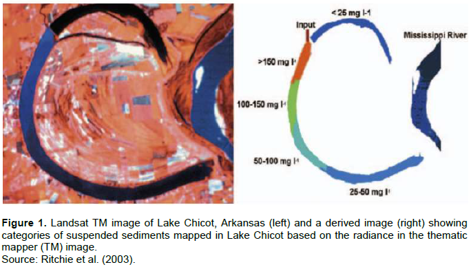
Schiebe et al. (1992) used this equation to estimate suspended sediments concentrations in Lake Chicot, Arkansas. According to Schiebe et al. (1992) study, it can be concluded that surface suspended sediments can be mapped and monitored in large water bodies using sensors available on current satellites. Figure 1 is a display of the Landsat TM image of Lake Chicot, Arkanas (left) and a derived image (right) showing categories of suspended sediments.
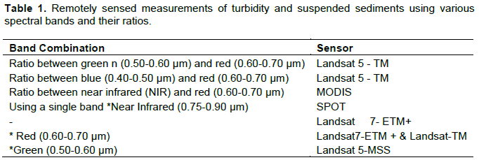
According to the Environmental Protection Agency, these are the key pollutants which affect water quality, which estimated that at least 40% of the waters, globally, do not meet the minimum water quality standards (Kuwayama et al., 2020). Academics have, in the recent years assumed and concluded that suspended sediments are the most common pollutants in sub-basins (Hirave et al., 2021; Novotny and Chesters, 1989; Wilber and Clarke, 2001). Curran and Novo (1988), in a review of the remote sensing of suspended sediments, found that optimum wavelength was related to suspended sediment concentration, thus high concentration of sediments has adverse impacts on the water quality of a sub-basin. The literature showed that turbidity and/or suspended sediments can be measured using visual spectral bands and various band ratios, which are summarized in Table 1.
Many studies have developed algorithms between the concentration of suspended sediments and reflectance for a specific date and geographic location (Kabir and Ahmari, 2020; Tavora et al., 2020; Yepez et al., 2018). However, few studies have further developed and used these algorithms to estimate suspended materials for future reference in time and space (Mertes et al., 1993). A curvilinear relationship between suspended sediments and reflectance has been established, the amount of reflected radiance tends to saturate as suspended sediment concentrations increase, thus identification of such contaminants is possible (Ritchie et al., 1990).
Chlorophyll/algae
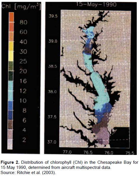
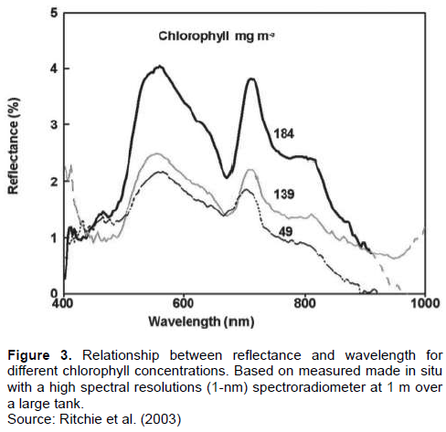
Remote sensing has been used to spatially measure chlorophyll concentrations spatially and temporally. As with suspended sediment measurements, most remote sensing studies of chlorophyll in water are based on empirical relationships between reflectance in narrow bands and chlorophyll. Measurements made in situ Ritchie et al. (2003) show spectra (Figure 2) with increasing reflectance with increased chlorophyll concentration across most wavelengths but areas of decreased reflectance in the spectral absorption region for chlorophyll (675 to 680 nm). A variety of algorithms and wavelengths have been used to successfully map chlorophyll concentrations of sub-basin waters. Harding Jr and Perry (1997) cited in Ritchie et al. (2003) used the following algorithm, Equation 2 based on aircraft measurements to determine seasonal patterns of chlorophyll content:

where a and b are empirical constant derived from in-situ measurements and G is [(R2)2 / (R1*R3)]. R1 is reflectance at 460 nm, R2 is reflectance at 490 nm, and R3 is radiance at 520 nm.
Previous studies have also indicated that the wavelength range for characterizing chlorophyll-a is between 400 and 900 nm (Han and Jordan, 2005). Thus, using this algorithm, Harding Jr and Perry (1997) mapped and displayed chlorophyll content as pollutants in a river basin. While estimating chlorophyll using remote sensing techniques is possible, studies have also shown that the broad wavelength spectral data available on current satellites such as Landsat and SPOT imagery, do not permit discrimination of chlorophyll in waters with high suspended sediments due to the dominance of the spectral signal from suspended sediments (Ritchie et al., 2003; Kutser, 2004; Olmanson et al., 2015; Gholizadeh et al., 2016).
Using this algorithm, Harding Jr and Perry (1997) cited in Ritchie et al. (2003), mapped total chlorophyll content in the Chesapeake Bay, United States of America (USA), as shown in Figure 2. Ritchie et al. (2003) also demonstrated, graphically, the relationship between reflectance and wavelength for different chlorophyll concentrations in in Figure 3.
Thus, the ability of remote sensing to identify pollutants such as chlorophyll/algae is quite limited, and these findings suggest new approaches for the application of airborne and spaceborne sensors to exploit these phenomena to estimate chlorophyll in surface waters (Iriarte Ahon, 1996). Our ability as researchers and policymakers, to monitor chlorophyll and associated pollutants will improve as hyperspectral and improved spatial data become readily available (Chang et al., 2015). Among other algorithms, for the identification and quantification of chlorophyll/algae content in sub-basins, band ratioing has proven to be advantageous because it allows for the compensation of variations from atmospheric influences (Han and Jordan, 2005).
Temperature
Thermal pollution exists when biological activities are affected by the changing temperature of a water body by anthropogenic activity (Caissie, 2006). Thermal plumes in rivers and lakes can be accurately estimated by remote sensing techniques. Mapping of absolute temperature by remote sensing provides spatial and temporal patterns of thermal releases. Caissie (2006) further posits that, aircraft mounted thermal sensors are especially useful in studies of thermal plumes because of the ability to control the timing of data collection. Seasonal changes in the temperature of surface waters can be expected. Such seasonal changes of rivers and sub-basin surface temperatures have been routinely monitored using the AVHRR, which is the Advanced Very High Resolution Radiometer, a radiation detection imager that can be used for remotely determining cloud cover and the surface of the earth as well as the surface of a body of water (Gitas et al., 2004). This leads to new insights into the role which rivers and lakes play in regulating weather and climate (Cairns Jr, 1971; Ritchie and Schiebe, 2000; Ritchie et al., 2003). Miller and Rango (1984) used a Heat Capacity Mapping Mission (HCMM) data to map emitted thermal energy and algae concentration in the Great Salt Lake, Northern Utah, in the United States.
A positive correlation during the day and a negative correlation at night between emitted energy and algal concentration was established (Ritchie et al., 2003). Ritchie et al. (1990) estimated surface temperatures of lakes along the Mississippi River using thermal data from Landsat Thematic Mapper. Thermal remote sensing is a useful tool for monitoring freshwater systems to detect thermal changes that can affect biological productivity. These techniques allow the development of management plans to reduce the effect of man-made thermal releases. The following equation was used by Ling et al. (2017), to estimate and determine surface water temperature for thermal pollution identification in sub-basin waters. Digital numbers (DN) for each water pixel in the band 6 (low gain) of Landsat ETM+ scenes were then used to derive water surface temperatures. First, digital numbers were converted to Top of Atmospheric (TOA) spectral radiance by applying the gain and bias coefficients as indicated in Equation 3 provided along with Landsat ETM+ scenes (Ritchie et al., 2003):
where Lλ is the TOA spectral radiance at λ wavelength in W·m2 · sr · mm, DN is the digital number in the scene, and gain and bias are calibration parameters, and are set to be 0.067087 and −0.07 for the band 6 (low gain) of Landsat 7 ETM+ images (Ritchie et al., 2003).
Long term in-situ water temperature records were a popular method to evaluate the influence of thermal pollution caused by climate change. In-situ records are always measured only at sparse certain locations and cannot provide detailed spatial information for thermal pollution assessment (Ling et al., 2017). By contrast, Landsat ETM+ and the advanced very high-resolution radiometer (AVHRR), thermal infrared imagery can provide long term spatially continuous water temperatures (Politi et al., 2012), which could then be used as an alternative dataset to assess the thermal pollution for large rivers and sub-basins, as presented in Figure 4. Surface temperatures of Lake Baikai derived from the Advanced Very High-Resolution Radiometer band 4 for 04 September 1991 (Figure 4).
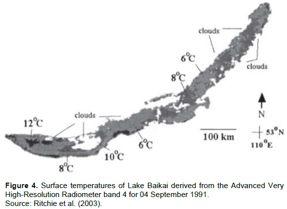
The spatial resolution of thermal imagery is a crucial factor that affects the accuracy of the estimated water temperature from thermal imagery (Anderson et al., 2012). In general, in order to estimate river water temperature accurately, the rivers should be as large as three pixels in the thermal infrared imagery (Sentlinger et al., 2008; Ling et al., 2017). However, if image sharpening methods are applied, water temperatures in the rivers narrower than the pixel size may also be estimated and used to identify the along-stream temperature pattern (Ling et al., 2017). Landsat ETM+ thermal images, which have a spatial resolution of 60 m, are suitable to be applied to estimate the water temperature (Handcock et al., 2006). In other cases, if Landsat 5 TM thermal imagery with a spatial resolution of 120 m or the Landsat 8 thermal imagery with a spatial resolution of 100 m, are used, or the river width is not large enough, these advanced water temperature algorithms should be used to improve the accuracy of results (Handcock et al., 2006; Ling et al., 2017).
Selected remote sensing techniques/algorithms for pollutant identification
While current remote sensing technologies have many actual and potential applications for assessing water resources and for monitoring water quality, limitations in spectral and spatial resolution of current sensors on satellites currently restrict the wide application of satellite data for monitoring water quality and precisely identifying and measuring pollutant distribution in sub-basins (Glasgow et al., 2004; Sheffield et al., 2018). In hindsight, the equations which assist in pollutant identification would work well if they can be incorporated with land use/land cover thematic maps as this would assist in identifying the distribution, pattern and direction of the pollutants, such as suspended sediments. However, this would be difficult in this case of thermal pollution where the temperature of the water is relatively high and changes the physio-chemical parameters and elements of water.
Therefore, the strength of remote sensing techniques remains in their capacity to deliver both spatial and temporal views of surface water quality parameters that is typically not possible from in situ measurements (Giardino et al., 2010; Ritchie and Schiebe, 2000). Remote sensing makes it possible to monitor the landscape effectively and efficiently, identifying water bodies with significant water quality problems. The Landsat 7 ETM sensor offers several enhancements over the Landsat 5 TM sensor (Chen et al., 2003), including increased spectral information content, improved geodetic accuracy, reduced noise, reliable calibration, improved spatial resolution of the thermal band from 120 to 60 m, and double thermal bands in the 10.40 to 12.5 mm window: band of 10.3 to 11.3 mm and band 11.5 to 12.5 mm (Chen et al., 2003; Wulder et al., 2019). The thermal data of Landsat 7 is expected to improve the accuracy of thermal pollution investigation and provide more detailed distribution pattern of thermal pollution.
Artificial neural networks for water pollutant identification in sub-basins
Dissolved oxygen
Identification and quantification of dissolved oxygen (DO) profiles of river is one of the primary concerns for water resources managers, hence is a water quality parameter and pollutant which requires artificial neural networks for identification, quantification and analysis (Najah et al., 2013). Several DO models such as deterministic and stochastic models have been developed in order to manage the best practices for conserving the DO in water bodies (Wen et al., 2013). Most of these models are complex and need several different input data which are not easily accessible, making it a very expensive and time-consuming process (Wen et al., 2013). Artificial neural networks (ANNs) are flexible modelling tools with the capability of learning the mathematical mapping between input and output variables of nonlinear systems and generalizing the processes of control, classification, and prediction (Govindaraju, 2000; Maier and Dandy, 2000).
In a study conducted in China by Wen et al. (2013), river water quality was tested using artificial neural network algorithms for the identification and quantification of dissolved oxygen. In view of the requirements of the neural computation algorithm, the raw data of both the input and output variables must be normalized to an interval by transformation. All the variables were normalized ranging from -1 to 1 using Equation 4 (Wen et al., 2013):
where xn and xi represent the normalized and original training, test, and validation data; x min and x max denote the minimum and maximum of the training, test, and validation data (Wen et al., 2013).
River and sub-basin dissolved oxygen concentration can be defined as a complex phenomenon affected by factors that are ever changing (Moridi, 2019; Ouma et al., 2020), some of which may not entirely be captured by traditional laboratory measurement techniques. Dissolved oxygen concentration in rivers was not constant even under the most stable atmospheric conditions such as temperature, rainfall, and wind velocity, among others (Du and Shen, 2015; Whitehead et al., 2009).
Therefore, increasing the water quality parameters under consideration improves the artificial neural network model performance by bringing into view other factors that may not have been considered before (Alizadeh and Kavianpour, 2015). From the moving average trend line in Figure 5, there is an indication that the general trend in the DO concentration within the basin is decreasing.
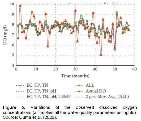
The study results showed that in the prediction of DO using water quality parameters, optimal results were obtained by combining temperature, electric conductivity, total phosphorus, pH, and total nitrates as the predictor variables for ANN models, with correlation coefficients R = 0.8425 and R = 0.5703, respectively (Ouma et al., 2020).
CONCLUSION
From the available literature, a pertinent deduction is that various space and airborne sensors can measure water quality parameters and pollutants in sub-basins with reliable precision. In most cases, managers and policy makers without technical expertise typically lack the knowledge to understand technical descriptions, abilities and limitations of remote sensing-based techniques and algorithms, as well as that of artificial neural networks. Therefore, this paper has a significant contribution to the study of remote sensing and artificial neural network methodology and the ability of these methodologies to identify and quantify pollutant distribution in sub-basins. It is highly recommended that researchers, who work in the field of optics and remote sensing, continue to communicate more with water resource management agencies on using appropriate and available tools to address important water quality monitoring requirements. The equations presented in this paper, have in common the fact that, although developed some years ago, they are still relevant to the studies and application of water quality and pollutant identification.
The equations are of benefit to both academia and industry as they provide a way to synthesize various factors, indicating the identification, distribution, and quantification of microbial and physio-chemical pollutants in large water bodies.
Literature presented in this paper argued that in some cases, technologies, methods and algorithms are proven and readily available for use, however, in other cases, emergent technologies and approaches hold promise but require further field evaluation and cost reductions. It is, therefore, of critical importance to review and consider effective emergent technologies which will most effectively monitor progress towards the SDG 6 and water quality holistically. This will assist stakeholders to identify which kinds of policies and programs are working well collaboratively with water quality testing and the identification of pollutants in a basin, and which require corrective measures. Both remote sensing and artificial neural network-based algorithms, play a significant role in academic as well as in the field of work for the identification and quantification of pollutants in large water bodies. However, it would be of great benefit, to the community as well as to policy makers and water resource managers, to have simplified versions and explanations of pollutant identification and quantification equations, as this would encourage keeping sub-basin waters relatively clean and reduce reliance on chemicals for the purification of large water bodies for domestic, industrial and other uses.
CONFLICT OF INTERESTS
The authors have not declared any conflict of interests.
ACKNOWLEDGMENTS
Prof Raghavan Srinivasan and the SWAT team at TAMU Agrilife Research, USA, and Prof Ann Van Griensven and her research team, Department of Hydrology and Hydraulic Engineering, The Vrije University, Brussel, Belgium, are all sincerely acknowledged. Durban University of Technology is sincerely acknowledged for hosting the grant while University of The Western Cape is sincerely acknowledged for hosting the students who are supported by this grant. This work was supported by the South African National Research Foundation [grant numbers UID 116021, 2019]; the BRICS multilateral R&D project [grant number BRICS2017-144]; and the Durban University of Technology UCDG Water Research Focus Area grant.
REFERENCES
|
Aldhyani TH, Al-Yaari M, Alkahtani H, Maashi M (2020). Water Quality Prediction Using Artificial Intelligence Algorithms. Applied Bionics and Biomechanics, 2020. |
|
|
Alizadeh MJ, Kavianpour MR (2015). Development of wavelet-ANN models to predict water quality parameters in Hilo Bay, Pacific Ocean. Marine Pollution Bulletin 98(1-2):171-178. |
|
|
Almuktar S, Hamdan ANA, Scholz M (2020). Assessment of the effluents of Basra City main water treatment plants for drinking and irrigation purposes. Water 12(12):3334. |
|
|
Anderson MC, Allen RG, Morse A, Kustas WP (2012). Use of Landsat thermal imagery in monitoring evapotranspiration and managing water resources. Remote Sensing of Environment 122:50-65. |
|
|
Bartram J, Balance R (1996). Water quality monitoring-A Practical guide to the design and implementation of freshwater. Quality Studies and Monitoring Programmes, United Nations Environment Programme and the World Health Organization (UNEP/WHO). |
|
|
Behmel S, Damour M, Ludwig R, Rodriguez M (2016). Water quality monitoring strategies-A review and future perspectives. Science of the Total Environment 571:1312-1329. |
|
|
Biswas AK, Tortajada C (2011). Water quality management: An introductory framework. International Journal of Water Resources Development 27(1):5-11. |
|
|
Cairns Jr J (1971). Thermal pollution: a cause for concern. Journal (Water Pollution Control Federation) pp. 55-66. |
|
|
Caissie D. (2006). The thermal regime of rivers: a review. Freshwater Biology 51(8):1389-1406. |
|
|
Carolita I, Trisakti B, Noviar H (2013). Environmental quality changes of singkarak water catchment area using remote sensing data. International Journal of Remote Sensing and Earth Sciences 10(2). |
|
|
Chang NB, Imen S, Vannah B (2015). Remote sensing for monitoring surface water quality status and ecosystem state in relation to the nutrient cycle: a 40-year perspective. Critical Reviews in Environmental Science and Technology 45(2):101-166. |
|
|
Chawla I, Karthikeyan L, Mishra AK (2020). A review of remote sensing applications for water security: Quantity, quality, and extremes. Journal of Hydrology 585:124826. |
|
|
Chen C, Shi P, Mao Q (2003). Application of remote sensing techniques for monitoring the thermal pollution of cooling-water discharge from nuclear power plant. Journal of Environmental Science and Health Part A 38(8):1659-1668. |
|
|
Cid FD, Antón RI, Pardo R, Vega M, Caviedes-Vidal E (2011). Modelling spatial and temporal variations in the water quality of an artificial water reservoir in the semiarid Midwest of Argentina. Analytica Chimica Acta 705(1-2):243-252. |
|
|
Curran P, Novo E (1988). The relationship between suspended sediment concentration and remotely sensed spectral radiance: a review. Journal of Coastal Research pp. 351-368. |
|
|
de Paul Obade V, Moore R (2018). Synthesizing water quality indicators from standardized geospatial information to remedy water security challenges: a review. Environment international 119:220-231. |
|
|
Department of Environmental Affairs and Development (DEAP) (2011). Management (IWRM) Action Plan: Status Quo Report Final Draft, Western Cape Integrated Water Resource. Provincial Government, Department of Environmental Affairs and Development Planning, South Africa. |
|
|
Du J, Shen J (2015). Decoupling the influence of biological and physical processes on the dissolved oxygen in the Chesapeake Bay. Journal of Geophysical Research: Oceans 120(1):78-93. |
|
|
El-Rawy M, Fathi H, Abdalla F (2019). Integration of remote sensing data and in situ measurements to monitor the water quality of the Ismailia Canal, Nile Delta, Egypt. Environmental Geochemistry and Health pp. 1-20. |
|
|
Georgakakos AP (n.d.). A Decision Support System for Integrated Water Resources Planning and Management in the Nile Basin. |
|
|
Gholizadeh MH, Melesse AM, Reddi L. (2016). A comprehensive review on water quality parameters estimation using remote sensing techniques. Sensors 16(8):1298. |
|
|
Giardino C, Bresciani M, Villa P, Martinelli A (2010). Application of remote sensing in water resource management: the case study of Lake Trasimeno, Italy. Water Resources Management 24(14):3885-3899. |
|
|
Gitas IZ, Mitri GH, Ventura G (2004). Object-based image classification for burned area mapping of Creus Cape, Spain, using NOAA-AVHRR imagery. Remote Sensing of Environment 92(3):409-413. |
|
|
Giupponi C, Giove S, Giannini V (2013). A dynamic assessment tool for exploring and communicating vulnerability to floods and climate change. Environmental Modeling and Software 44:136-147. |
|
|
Glasgow HB, Burkholder JM, Reed RE, Lewitus AJ, Kleinman JE (2004). Real-time remote monitoring of water quality: a review of current applications, and advancements in sensor, telemetry, and computing technologies. Journal of Experimental Marine Biology and Ecology 300(1-2):409-448. |
|
|
Gleick PH (2000). A look at twenty-first century water resources development. Water International 25(1):127-138. |
|
|
Gorde S, Jadhav M (2013). Assessment of water quality parameters: a review. J Eng Res Appl 3(6):2029-2035. |
|
|
Govindaraju RS. (2000). Artificial neural networks in hydrology. II: hydrologic applications. Journal of Hydrologic Engineering 5(2):124-137. |
|
|
Greenfield R (2019). An assessment of the impacts of municipal wastewater from the Lydenburg wastewater treatment works, Mpumalanga, South Africa. |
|
|
Han L, Jordan KJ (2005). Estimating and mapping chlorophyll?a concentration in Pensacola Bay, Florida using Landsat ETM+ data. International Journal of Remote Sensing 26(23):5245-5254. |
|
|
Handcock R, Gillespie A, Cherkauer K, Kay J, Burges S, Kampf S (2006). Accuracy and uncertainty of thermal-infrared remote sensing of stream temperatures at multiple spatial scales. Remote Sensing of Environment 100(4):427-440. |
|
|
Harding Jr L, Perry E (1997). Long-term increase of phytoplankton biomass in Chesapeake Bay, 1950-1994. Marine Ecology Progress Series 157:39-52. |
|
|
Herrera V (2019). Reconciling global aspirations and local realities: Challenges facing the Sustainable Development Goals for water and sanitation. World Development 118:106-117. |
|
|
Hirave P, Glendell M, Birkholz A, Alewell C (2021). Compound-specific isotope analysis with nested sampling approach detects spatial and temporal variability in the sources of suspended sediments in a Scottish mesoscale catchment. Science of the Total Environment 755:142916. |
|
|
Hossain MD, Chen D (2019). Segmentation for Object-Based Image Analysis (OBIA): A review of algorithms and challenges from remote sensing perspective. ISPRS Journal of Photogrammetry and Remote Sensing 150:115-134. |
|
|
Igbinosa E, Okoh A (2009). Impact of discharge wastewater effluents on the physico-chemical qualities of a receiving watershed in a typical water radiance and suspended sediment concentration using digital rural community. International Journal of Environmental Science and Technology 6(2):175-182. |
|
|
Iriarte Ahon F (1996). Satellite applications as an ocean and coastal zone management tool: three cases studies. |
|
|
Kabir SMI, Ahmari H (2020). Evaluating the effect of sediment color on imagery. Journal of Hydrology 589:125189. |
|
|
Kapalanga TS, Hoko Z, Gumindoga W, Chikwiramakomo L (2020). Remote sensing-based algorithms for water quality monitoring in Olushandja Dam, north-Central Namibia. Water Supply. |
|
|
Krenkel P. (2012). Water quality management: Elsevier. |
|
|
Kutser T (2004). Quantitative detection of chlorophyll in cyanobacterial blooms by satellite remote sensing. Limnology and Oceanography 49(6):2179-2189. |
|
|
Kuwayama Y, Olmstead SM, Wietelman DC, Zheng J (2020). Trends in nutrient-related pollution as a source of potential water quality damages: A case study of Texas, USA. Science of the Total Environment 724:137962. |
|
|
Ling F, Foody GM, Du H, Ban X, Li X, Zhang Y, Du Y (2017). Monitoring thermal pollution in rivers downstream of dams with Landsat ETM+ thermal infrared images. Remote Sensing 9(11):1175. |
|
|
Luo Y, Ficklin DL, Liu X, Zhang M (2013). Assessment of climate change impacts on hydrology and water quality with a watershed modeling approach. Science of the Total Environment 450:72-82. |
|
|
Maier HR, Dandy GC (2000). Neural networks for the prediction and forecasting of water resources variables: a review of modelling issues and applications. Environmental Modelling and Software 15(1):101-124. |
|
|
Mertes LA, Smith MO, Adams JB (1993). Estimating suspended sediment concentrations in surface waters of the Amazon River wetlands from Landsat images. Remote sensing of Environment 43(3):281-301. |
|
|
Miller W, Rango A (1984). Using heat capacity mapping mission (hcmm) data to assess lake water quality 1. Journal of the American Water Resources Association 20(4)493-501. |
|
|
Moridi A. (2019). Dealing with reservoir eutrophication in a trans-boundary river. International Journal of Environmental Science and Technology 16(7):2951-2960. |
|
|
Najah A, El-Shafie A, Karim OA, El-Shafie AH (2013). Application of artificial neural networks for water quality prediction. Neural Computing and Applications 22(1):187-201. |
|
|
Novotny V, Chesters G. (1989). Delivery of sediment and pollutants from nonpoint sources: a water quality perspective. Journal of Soil and Water Conservation 44(6):568-576. |
|
|
Oliver S, Corburn J, Ribeiro H (2019). Challenges regarding water quality of eutrophic reservoirs in urban landscapes: a mapping literature review. International Journal of Environmental Research and Public Health 16(1):40. |
|
|
Olmanson LG, Brezonik PL, Bauer ME (2015). Remote sensing for regional lake water quality assessment: capabilities and limitations of current and upcoming satellite systems. In Advances in watershed science and assessment: Springer pp. 111-140 |
|
|
Osibanjo O, Daso AP, Gbadebo AM (2011). The impact of industries on surface water quality of River Ona and River Alaro in Oluyole Industrial Estate, Ibadan, Nigeria. African Journal of Biotechnology 10(4):696-702. |
|
|
Ouma YO, Okuku CO, Njau EN (2020). Use of artificial neural networks and multiple linear regression model for the prediction of dissolved oxygen in rivers: case study of hydrographic basin of River Nyando, Kenya. Complexity, 2020. |
|
|
Oxford M (1976). Remote sensing of suspended sediments in surface waters. Photogramm. Eng. Remote Sens 42:1539-1545. |
|
|
Palmer SC, Kutser T, Hunter PD (2015). Remote sensing of inland waters: Challenges, progress and future directions. In: Elsevier. |
|
|
Pierson DC, Strömbeck N (2000). A modelling approach to evaluate preliminary remote sensing algorithms: Use of water quality data from Swedish Great Lakes. Geophysica 36(1-2):177-202. |
|
|
Politi E, Cutler ME, Rowan JS. (2012). Using the NOAA Advanced Very High Resolution Radiometer to characterise temporal and spatial trends in water temperature of large European lakes. Remote Sensing of Environment 126:1-11. |
|
|
Rawat KS, Singh SK, Gautam SK (2018). Assessment of groundwater quality for irrigation use: a peninsular case study. Applied Water Science 8(8):1-24. |
|
|
Ritchie JC, Schiebe FR (2000). Water quality. In Remote sensing in hydrology and water management (pp. 287-303): Springer. |
|
|
Ritchie JC, Zimba PV (2006). Estimation of suspended sediment and algae in water bodies. Encyclopedia of hydrological sciences. |
|
|
Ritchie JC, Cooper CM, Schiebe FR (1990). The relationship of MSS and TM digital data with suspended sediments, chlorophyll, and temperature in Moon Lake, Mississippi. Remote Sensing of Environment 33(2):137-148. |
|
|
Ritchie JC, Cooper CM, Yongqing J (1987). Using Landsat multispectral scanner data to estimate suspended sediments in Moon Lake, Mississippi. Remote sensing of Environment 23(1):65-81. |
|
|
Ritchie JC, Zimba PV, Everitt JH (2003). Remote sensing techniques to assess water quality. Photogrammetric Engineering and Remote Sensing 69(6):695-704. |
|
|
Schiebe F, Harrington Jr J, Ritchie J (1992). Remote sensing of suspended sediments: the Lake Chicot, Arkansas project. International Journal of Remote Sensing 13(8):1487-1509. |
|
|
Schmugge TJ, Kustas WP, Ritchie JC, Jackson TJ, Rango A (2002). Remote sensing in hydrology. Advances in Water Resources 25(8-12):1367-1385. |
|
|
Scott G, Rajabifard A (2017). Sustainable development and geospatial information: a strategic framework for integrating a global policy agenda into national geospatial capabilities. Geo-spatial information science 20(2):59-76. |
|
|
Sentlinger GI, Hook SJ, Laval B (2008). Sub-pixel water temperature estimation from thermal-infrared imagery using vectorized lake features. Remote sensing of Environment 112(4):1678-1688. |
|
|
Sheffield J, Wood EF, Pan M, Beck H, Coccia G, Serrat?Capdevila A, Verbist K (2018). Satellite remote sensing for water resources management: Potential for supporting sustainable development in data?poor regions. Water Resources Research 54(12):9724-9758. |
|
|
Tavora J, Boss E, Doxaran D, Hill P (2020). An algorithm to estimate suspended particulate matter concentrations and associated uncertainties from remote sensing reflectance in coastal environments. Remote Sensing 12(13):2172. |
|
|
Wen X, Fang J, Diao M, Zhang C (2013). Artificial neural network modeling of dissolved oxygen in the Heihe River, Northwestern China. Environmental Monitoring and Assessment 185(5):4361-4371. |
|
|
Whitehead PG, Wilby RL, Battarbee RW, Kernan M, Wade AJ (2009). A review of the potential impacts of climate change on surface water quality. Hydrological Sciences Journal 54(1):101-123. |
|
|
Wilber DH, Clarke DG (2001). Biological effects of suspended sediments: a review of suspended sediment impacts on fish and shellfish with relation to dredging activities in estuaries. North American Journal of Fisheries Management 21(4):855-875. |
|
|
Wulder MA, Loveland TR, Roy DP, Crawford CJ, Masek JG, Woodcock CE, Cohen WB (2019). Current status of Landsat program, science, and applications. Remote Sensing of Environment 225, 127-147. |
|
|
Yepez S, Laraque A, Martinez JM, De Sa J, Carrera JM, Castellanos B, Lopez JL (2018). Retrieval of suspended sediment concentrations using Landsat-8 OLI satellite images in the Orinoco River (Venezuela). Comptes Rendus Geoscience 350(1-2):20-30. |
|
Copyright © 2024 Author(s) retain the copyright of this article.
This article is published under the terms of the Creative Commons Attribution License 4.0


