ABSTRACT
Abortive boreholes and parched wells, ascribed to the difficulty in understanding the hydrogeology of the aquifer by water borehole drillers, pose great concern to the people of the region. Mapping the spatial variability of water table depth (WTD) (m) and aquifer thickness H (m) is a vital step in optimal utilization of groundwater resources. Thus, the aim of this paper is to investigate the spatial variability of the groundwater parameters, H (m) and WTD (m) in the study area located in Nigeria, using geostatistical method of Ordinary Kriging, based on data estimated from interpreted results of fifty (50) Schlumberger Vertical Electrical Sounding (VES) curves. To attain this aim, the spatial variability of the groundwater parameters was analyzed. The result shows that the difference in directional behavior is not significant. Thus, the WTD and H were assumed as isotropic, and experimental semivariograms of logH and log(WTD) were calculated and modeled with the GS+ software. It was found that, H and (WTD) data are moderately spatially correlated over the study area, and the spatial structures follow exponential model for H and spherical model for (WTD). According to the generated maps of kriged estimates of logH and log(WTD), the southern part of the study area with higher prolific aquiferous zone, shows higher kriged H-values, relative to the northern zone. The variation in the distribution of kriged WTD-values in the study region is asymmetrical. These results compare favorably in the trend patterns of distribution of the parameter values, with contour maps of a previous study in the region that indicates the distribution of H and WTD parameters. The parameters of the semivariogram models used for the analysis of the data, give insight into the spatial pattern of the groundwater parameters, H and WTD. This knowledge has improved the ability to understand the hydrogeology of the aquifer. The generated spatial variability maps of H and WTD will assist water resource managers and policymakers in the development of guidelines in judicious management of groundwater resources for drinking purposes in the study area.
Key words: Ordinary kriging, Aquifer thickness, water table depth, semivariogram, exponential model, spherical model, cross-validation.
In recent years, the importance of groundwater as a natural resource has been increasingly recognized throughout the world. But, population growth in the study area has resulted in expanding residential developments and consequently, increased demand for water, resulting in lowering of the groundwater water table due to excessive withdrawals.Keeping the water table at a favorable level is quite significant. When a well is placed in an aquifer, lowering the water table will not only have an effect on the thickness of the aquifer, but can also cause salt water from the ocean to move further inland, acting as a contaminant to aquifers. As the water table becomes too low to be tapped from, the expensive wells are abandoned as unproductive or desiccated wells. Therefore, it is very important to estimate the spatial distribution pattern of the groundwater aquifer parameters in order to boost the ability to understand the fluctuations in water table depth due to extraction and the hydrogeology of the aquifer. Using geostatistics, it is possible to map the spatial variability of the aquifer parameters and improve the qualitative and quantitative management of water resources. This has been described further with literature review. For example, Ahmadi and Sedghamiz (2007) evaluated kriging and cokriging methods for mapping the groundwater depth across a plain in which there has been different climatic conditions (dry, wet, and normal). Results obtained from geostatistical analysis showed that groundwater depth varied spatially in different climatic conditions. Yang et al. (2008) discussed the kriging approach combined with hydrogeological analysis (based on GIS) for the design of groundwater level monitoring network. The effect of variogram parameters (that is, the sill, nugget effect and range) on network was analyzed. In their efforts to analyze the spatial variability of groundwater depth and quality parameters, Dash et al. (2010), used ordinary kriging and indicator kriging to generate spatial variability maps in the National Capital Territory of Delhi, India. The results indicated that in 43% of the study area, groundwater depth was within 20 m. The salinity level was higher than 2.5 ds m−1 in 69% of the study area. Also, Andarge et al. (2013), estimated transmissivity using empirical and geostatistical methods in the volcanic aquifers of Upper Awash Basin, Central Ethiopia. They performed linear and logarithmic regression functions and it was found that the logarithmic relationship predicting transmissivity from specific capacity data has a better correlation (R = 0.97) than the linear relationship (R = 0.79). Masoomeh et al. (2013), investigated the spatio-temporal variability of groundwater quality parameters (Electrical Conductivity, Sodium Adsorption Ratios, Total Dissolved Solids, and Sodium content) using geostatistics and GIS in Shiraz City, South Iran. Results revealed that ground water quality data are strongly spatially correlated over the study region. Pradipika and Surya (2014) studied the spatial variability of ground water depth and quality parameter in Haridwar District of Uttarakhand, using ordinary kriging. It was observed that the semivariogram parameters fitted well in the spherical model for water depth, and in the exponential model for water quality parameter. Both parameters followed a log-normal distribution and demonstrated a moderate spatial dependence according to the nugget ratio. Other similar studies have shown that geostatistical approach is a suitable method for estimation of aquifer hydraulic properties (Doctor and Nelson, 1981; Sophocleous et al., 1982; Nunes et al., 2004a; Arslan, 2012, 2013; Rawat et al., 2012; Varouchakis et al., 2012; Delbari, 2013). Thus, to achieve the purpose of this study, the core objectives consists of variographic analysis of the spatial variability of groundwater parameters H and WTD, the generation of maps of kriged estimates of logH and log(WTD), and back transforms of logH and log(WTD) to H and WTD to assess the H and WTD fields.
Description of study area
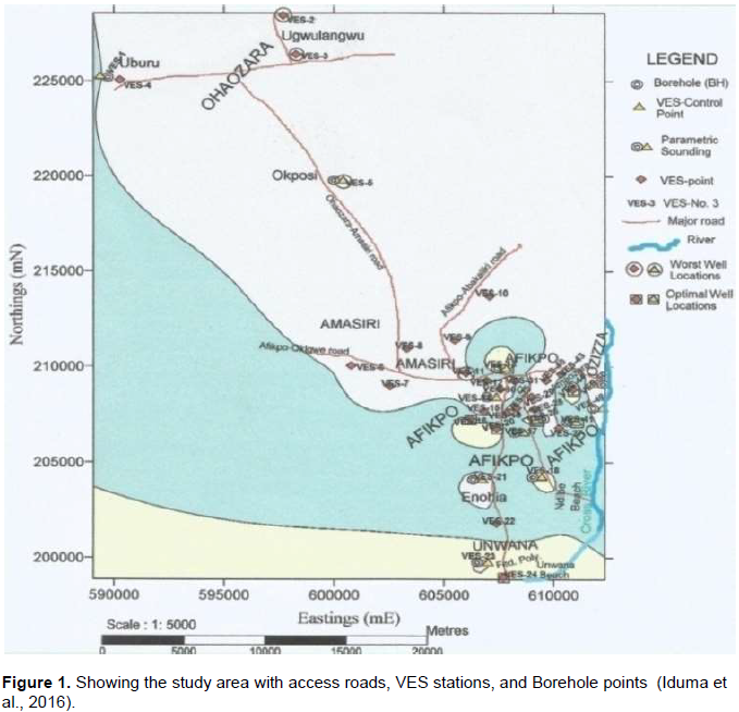
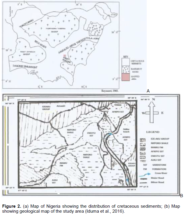
The study area falls within Southeastern Nigeria in the Afikpo Basin, bounded by Long. 7° 45′E to 8° 00′E and Lat. 5° 43′N to 5° 57′N (in Nigerian local datum) and traverses two regions; the Ohaozara area and Afikpo province-consisting of Amasiri, Ozziza, and Unwana, covering an area of about 607.75 km2 (Figure 1). The area lies mostly in the (Eboine) River Basin and the Cross River plains on the south-eastern flank of the Abakaliki-Benue anticlinorium (Figure 2a). The area has an undulating terrain and an elevation of about 170 m above mean sea level. Remarkably, sandstone forms its ridges and the shale forms the valley. The shale unit underlies the bioturbated sandstone. These bioturbated sandstones have very high altitude; this is possibly because they have less period of exposure to erosion.
Geology and hydrogeology of the study area
Geologically, the area falls within the Cretaceous Abakaliki-Benue Rift (Figure 2a), and is underlain by the Asu River Group (Albian), the Turonian Eze-Aku formation and the (Late Campanian-Early Maastrichtian) Nkporo formation. The Turonian Amasiri sandstone of the Eze-Aku group is a highly consolidated, well cemented, subangular to subrounded, poorly sorted, very fine to medium grained feldspathic arenite with poor reservoir quality (Okereke, 2012). This unit dominates the northern parts of the study area. Local geology of the study area indicates that extensive marine transgression and regression occurred in the Turonian followed by the period of Orogeny during the Coniancian, especially the Santonian. Contemporaneous with the Orogeny was the intrusion of the igneous bodies described as dolerite sills, into the Eze-Aku Shale (Okonkwo et al., 2013; Obiora, 2002). The geological map of the study area is as shown in Figure 2b. The Nkporo Formation is the basal lithostratigraphic unit of the Afikpo sub-basin and comprises dominantly of dark grey to black shales, sandstone, minor limestone and oolitic ironstone beds. In the Campanian-Maastrichtian, there was subsidence and a marine regression resulted in the deposition of a lateral equivalent to Nkporo Formation named Afikpo Sandstone. Simpson (1954), Reyment (1965) and Whiteman (1982) reported the presence of an angular unconformity between the Campanian-Maastrichtian Afikpo Sandstone and the Turonian Eze-Aku group. The Afikpo Sandstone is the youngest sedimentary unit in the study area. Its relatively loose structure, coarse grains, sorting enables it to be porous and permeable. The formation covers most parts of Afikpo town, hence the name, Afikpo Sandstone. Shale and sandstone are the two major lithologic units in the area. The sandstone units constitute the permeable and saturated aquifers. The dominant lithology in the southern zone of the study is the Afikpo sandstone. Almost, the entire northern area is underlain by well compacted, hard Amasiri Sandstone of the Santonian Eze-Aku group. The nature of this unit obviously reduces infiltration unless in parts that are fractured or deeply weathered. It is possible that the regional Cretaceous tectonic activity shattered the rocks of the area after the deposition of the sediments. Hence, places that exhibit intense fracturing yield water at shallow depth (Simpson, 1955).
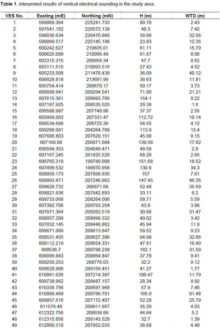
The geostatistical study is based on data estimated from interpreted results of fifty (50) Schlumberger Vertical Electrical Sounding (VES) curves with maximum current electrode spacing of AB/2 = 681 m. The details of the geoelectrical data acquisition, processing, and interpretation methods, are contained in Iduma (2014). For effective use of the geoelectrical data in the geostatistical study, the validity of the resistivity data was tested in a borehole-lithology and geoelectrical-column correlations. The H and WTD data values computed from the VES data are shown in Table 1. The procedures adopted in the correlation attempt are explained in Iduma et al. (2016).


Most often, skewed or erratic data can be made more suitable for geostatistical modeling by appropriate transformation. Ordinary kriging is well-known to be optimal when the data have a multivariate normal distribution. Transformation of data therefore may be required before kriging to normalize the data distribution, suppress outliers and improve data stationarity (Deutsch and Journel, 1992; Armstrong, 1989). The estimation then is performed in the Gaussian domain before back-transforming the estimates to the original domain. The Gaussian distribution has the advantage that spatial variability is easier to be modeled because it reduces the effects of extreme values providing more stable variograms (Goovaerts, 1997; Armstrong, 1989). In this study, geostatistical analysis of the data is accomplished using the software GS+ Ver. 10.0 (Gamma Design Software, Plainwell, USA). Fifty (50) aquifer thickness (H) and water table depth (WTD) data (Table 1), estimated from the interpretation of VES data were used as input data for the geostatistical study. Kriging represents variability only up to the second order moment (covariance), so the random field of the transformed variable must therefore be Gaussian to derive unbiased estimates at non-sampled locations (Deutsch and Journel, 1992; Goovaerts et al., 2005). A non-linear normalizing data transformation (log transformation) is applied in union with kriging for the accurate prediction of spatial variability of the groundwater parameters under study. A cross-validation (Isaaks and Srivastava, 1989) approach is used to assess the performance and interpolation errors of ordinary kriging in the estimation of groundwater parameters (H and WTD). The comparison criteria used are coefficient of determination (R2) and residual sum of squares (RSS). For appropriate estimator, R2 should be close to 1 and RSS should be as small as possible (Robertson, 2008). In this study, it is assumed that: (1) all values of (H) and WTD data, in the study area are the results of a random process, with dependence (spatial autocorrelation) and (2) the variance of the difference is the same between any two points that are at the same distance apart and direction, no matter which two points are chosen (stationarity assumption). The theory of geostatistics and principles of kriging have been well documented previously (Isaaks and Srivastava, 1989; Goovaerts, 1997; David, 1977; Journel and Huijbregts, 1978; Kitanidis, 1997) and will not be repeated in this paper. Interested readers are referred to these cited references. More advanced treatment of the subject can also be found in Webster and Oliver (2001).
Statistical analysis of H and WTD data has been presented. Spatial variability analysis and model fitting have been done. The results also include cross-validation and spatial prediction of H and WTD data, and mapped values of H and WTD with estimation variance maps.
Statistical analysis of H and WTD data
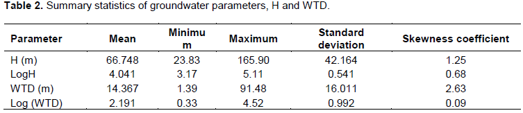
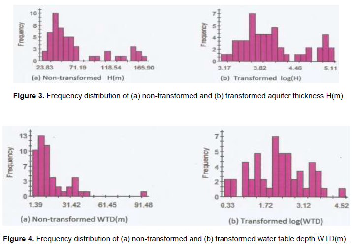
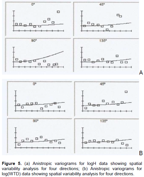
Table 2 provides descriptive statistics for H and WTD data. The available raw data range between 165.90 to 23.83 m and 91.48 to 1.39 m for H and WTD data, respectively, straddling several orders of magnitude. The mean values of H and WTD data are correspondingly, 66.748 and 14.367 m. To preserve a certain continuity of the data, some data values (outliers) were isolated relative to the entire data, in the cross-validation procedure. Figures 3b and 4b show the frequency distributions of logH and log(WTD), respectively, and indicate a fairly normal distribution relative to the untransformed, H and WTD data. The frequency distribution of the untransformed data is shown in Figures 3a and 4a. The frequency distribution of the transformed data is positively skewed with a symmetrical form. The skewness coefficient of transformed data (Table 2, column 6) is much less than those of real data. So, the data are transformed using a log transformation function. A comparison of standard deviation for log transformed data with the untransformed data for both parameters indicates that a reduction in prediction standard deviation would occur if log transformed H and WTD values are estimated against the untransformed data.
Spatial variability analysis and model fitting
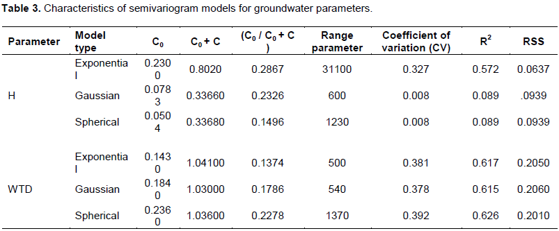
To investigate the spatial variability of groundwater parameters, experimental semivariograms of logH and log (WTD), are calculated for four directions (0, 45, 90 and 135°) with an angle tolerances of 22.5°. The results (Figure 5a and b), did not show any significance differences, that is, no significant anisotropy, hence, the investigated parameters are assumed to be isotropic, and omnidirectional semivariograms is calculated for each of them. Then the best semivariogram model is fitted to the experimental data. The model depends on the choice of three parameters: nugget, sill, and range parameters. The model fitting is done by defining a curve that provides the best fit through the points in the empirical semivariogram graph by ensuring that the squared difference (RSS) between the data points and the curve is minimum (Robertson, 2008). Spherical, Exponential, and Gaussian functions were fitted, one at a time, to the empirical data for evaluation. The best model, in bold letters (Table 3, column 2), is the one that has the least RSS and largest coefficient of variation (C.V), which is the square of correlation coefficient (R2). Semivariogram model characteristics for each parameter (H, WTD) are shown in Table 3. The fitting models to logH and log WTD experimental semivariograms are as shown in Figure 6a and b, respectively. As recommended by Mehrjardi et al. (2008), when the ratio C0 / (C0 +C) in Table 3, is less than 0.25, the variable has a strong spatial correlation, if the ratio C0 / (C0 +C) is greater than 0.25 and less 0.75, the variable has a moderate spatial correlation, but, when the ratio C0 / (C0 +C) is greater than 0.75, the variable is said to have a weak spatial correlation.
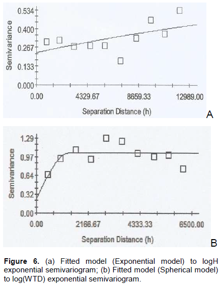
The results indicate that spatial structure of both variables, H and WTD, are moderate and follow an exponential model for the H data and spherical model for the WTD data.
Cross-validation and spatial prediction of H and WTD data
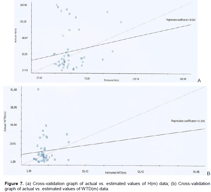
The semivariogram model characteristics shown in Table 3 are used in ordinary kriging to interpolate the groundwater parameters, logH and log(WTD) in the study area. The performance of the kriging-based geostatistical models is optimized by using the leave one out cross validation technique that is usually applied in small datasets (Witten et al., 2011). So, the models in Table 3 are further validated by a process of cross-validation. In the cross-validation procedure, each observed data point, one at a time, (leaving the model otherwise unaltered) is removed and the predicted value is computed at these points. In order to select the most valid model, this process is carried out for each of the three models. Each of the models (Gaussian, Exponential, and Spherical) was fitted, one at a time, on the logH and log(WTD) omnidirectional experimental semivariograms for appraisal. The true and estimated values of the cross-validation are compared using statistical measures. The best model is the one that has the highest regression coefficient (Robertson, 2008), in a cross-validation graph (graph of actual versus estimated values of the groundwater parameters, H and WTD). Regression coefficient represents a measure of the goodness of fit for the least-squares model describing the linear regression equation. A perfect 1:1 fit would have a regression coefficient (slope) of 1. The cross-validation graphs (Figure 7a and b), which compare the actual with the estimated values of H and WTD, respectively, indicate that exponential model with the highest regression coefficient (0.514), revealed in Figure 7a, is the best semivariogram model for the prediction of H data set, while the spherical model, with the highest regression coefficient (0.336), as shown in Figure 7b, is the best semivariogram model for the prediction of WTD data set in the study region.

The general approach that is used for interpolation applies a normalizing transformation followed by ordinary kriging on the transformed variable, and finally the predictions are back-transformed. In the kriging scheme, active lag distance of 12989 and 6500 m for H and WTD parameters, respectively, were specified with a minimum of 30 sample pairs (Istok and Copper, 1988), assured by identifying eight and ten as the minimum and maximum number of neighbors. The kriging system is completed within a round-shaped search neighborhood radius of 18.876 km (approximately half the maximum distance between sample points). The chosen semivariogram models shown in Figure 6a and b and described in Table 3, with the available log H and log(WTD) sample data were used to perform kriged estimation of logH and log(WTD) over the study area. Kriging system also calculates estimation variance or estimation standard deviation.
Mapped values of H and WTD data with estimation variance maps
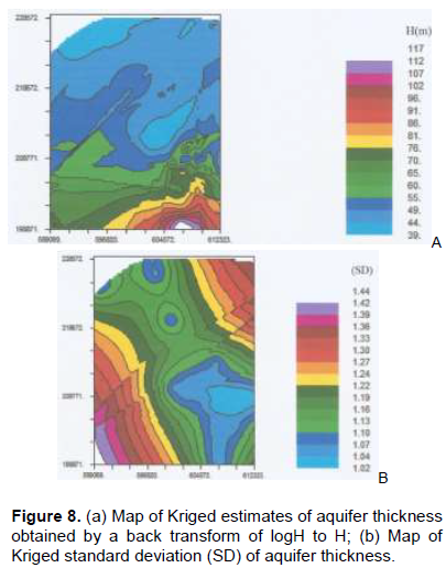
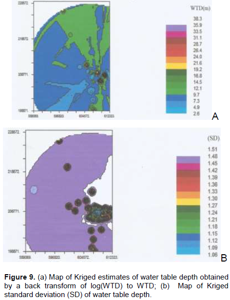
The kriged logH and log(WTD) maps are used subsequently, to make an estimation of H and WTD values over the study area through a back-transform of logH and log(WTD) to H and WTD. The maps of kriged estimates of H and WTD values which provide an assessment of the H and WTD values over the whole study region, are shown in Figures 8a and 9a, respectively. The estimation standard deviation maps in Figures 8b and 9b, corresponding to H and WTD values, present zones of weak and strong values, and indicate the quality of estimates. The smaller the standard deviation value, the higher the exactness of estimates. Due to border effect and the presence of zones where data points are deficient, highest values of standard deviations of estimates are found towards limits of the study area.
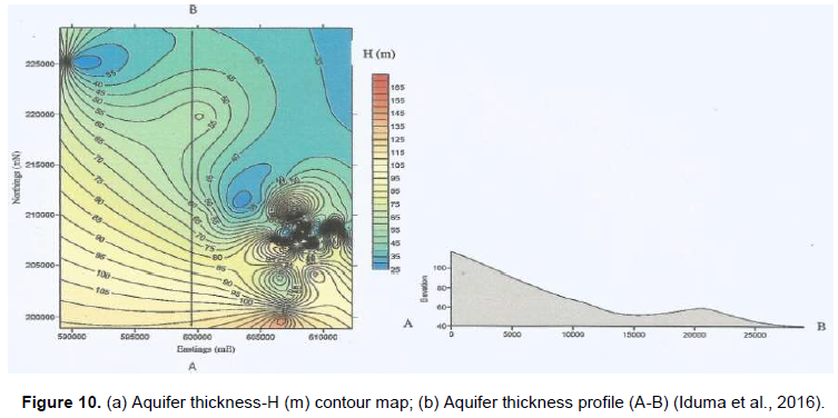
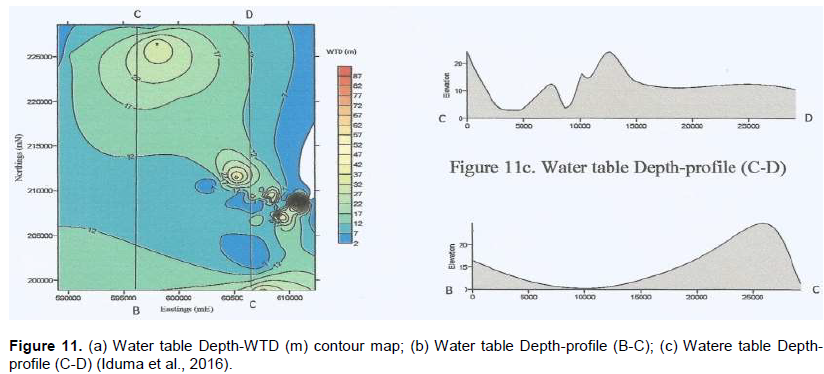
The ranges of experimental variograms of logH and log(WTD) are equal to 31.1 and 1.37 km, respectively (Table 3). These distances which indicate the scale of the spatial structure of the variables are significant. It means that two points in the field separated by a distance less than the range remain correlated with each other. For example, the distance 31.1 km, is the maximum distance over which the spatial dependence of the (H) variable becomes uncertain, hence, is a measure of the length of influence. The ratio of the nugget variance to the sill represents the importance of this influence (Holawe and Dutter, 1999). These large and small correlation lengths may be explained by patterns of undulation of the terrain in the study region. Of significance in this study is the large nugget effect (measurement error or error at small scale variability), which, in this case, indicates that spatial correlations between individual H and WTD parameters are not strong, but moderate, even at short distances. In practice, the nugget effect is the level of variability at dimensions less than the minimum sample spacing. So, the recognition of the level of nugget effect in association with the spatial range of influence has implications for prospective modelers in the study region. It becomes imperative that the potential modelers gain insight into the scales of spatial variation that might interest them before data collection. This is because variations at micro scales smaller than the sampling distances will appear as part of the nugget value. According to the generated maps, the southern part of the study area shows relatively higher kriged H-values. That may possibly, be attributed to the existence of Nkporo Formation which is comparatively the higher prolific aquiferous zone. The northern part of the region, underlain by a well compacted, hard Turonian Amasiri Sandstone of the Eze-Aku group is characterized by water scarcity, hence, the presence of relatively lower kriged H-values (Figure 8a). The variation in the distribution of kriged WTD-values in the study region is asymmetrical (Figure 9a). The irregular stretch of kriged WTD-values in the study region may plausibly, be ascribed to the undulating nature of the terrain (Hesse and MacDonald, 1975).The geostatistical procedure produced satisfactory distribution of high and low values of H and WTD in the study area, similar to available knowledge. In a previous study (Iduma et al., 2016) undertaken in the area, the contour maps (Figures 10a and 11a) of H and WTD, respectively, indicate similar distribution patterns. An isopach map of the aquiferous layer (Figure 10a) shows that aquifer thickness is highly variable, revealing a relatively progressive decrease in values of the aquifer thickness H, in the south-north direction. This condition is confirmed by the longitudinal profile A-B (Figure 10b), which shows a progressive decrease in values of the aquifer thickness H, in the south-north direction. Although the depth to water table tends to be low in some regions, and high in some other parts of the area, generally, the variation in the distribution of the WTD in the study area is irregular as shown in Figure 11a, and illustrated in the longitudinal profiles, BC and CD (Figure 11b and c, respectively).


A comparison of the maps of kriged estimates of H (Figure 8a) and WTD (Figure 9a) with the contour maps (Figures 10a and 11a) from previous study, indicates good agreement in the trend patterns of distribution of these parameter values in the study area. On this basis, the kriged estimates of the H and WTD data-values of the region could be understood to demonstrate coherence, and therefore prove to be reliable. It is pertinent to know that the logarithmic transforms of H and WTD to logH and log(WTD) are non-linear transforms. So, when the kriged unbiased estimates logH and log(WTD) are back-transformed, their unbiased properties are lost, and the H and WTD values estimated using this procedure are no longer unbiased.
Generally, results of this study showed that ordinary kriging which is best linear unbiased estimator, is the suitable method for estimation of groundwater parameters, H and WTD. By providing the variance of the estimation error, the method gives the quality of the estimation. The variographic analysis of both variables indicates that logH and log (WTD) are stationary variables, characterized by significant nugget effects (discontinuity at the origin of the variogram). Also, it could be concluded that the parameters of the semivariogram used for the structural description, give insight into the spatial pattern of the groundwater parameters, H and WTD. This knowledge has improved the ability to understand the hydrogeology of the study area. Additionally, this study has shown that ordinary kriging constitutes a reliable method to appraise the spatial autocorrelation of groundwater aquifer thickness and water table depth data in interpolation studies. The kriged-H and log(WTD) values are spread over several orders of magnitude, revealing the strong heterogeneity of these parameters in the study region. The generated spatial variability maps of H and WTD will assist water resource managers and policymakers in the development of guidelines in judicious management of groundwater resources for agricultural and drinking purposes in the study area.
The authors have not declared any conflict of interests.
The authors are deeply indebted to all authors whose works were consulted in the course of this project. They wish to express their appreciation to Mark Baylor, the sales team lead (Gamma Design Software-Plainwell, Michigan-USA) for making it possible to buy the Gamma Design software (15-digit Licence) at student's rate, and later helped to upgrade to 18-digit Licence and Michael Devine (Rockware, Inc. –Colorado USA) who provided the link to Gamma Design Software is also highly admired.
REFERENCES
|
Ahmadi S, Sedghamiz A (2007). Geostatistical analysis of spatial and temporal variations of groundwater Level. Environ. Monit. Assess. 129:277-294.
Crossref
|
|
|
|
Andarge YB, Moumtaz R, Tenalem A, Engida Z (2013). Estimating transmissivity using empirical and geostatistical methods in the volcanic aquifers of Upper Awash Basin, central Ethiopia. Environ. Earth Sci. 69(6):1791-1802.
Crossref
|
|
|
|
Armstrong M (1989). Review of the applications of geostatistics in the coal industry. Moscow: Kluwer Academic Publishers.
Crossref
|
|
|
|
Arslan H (2012). Spatial and temporal mapping of groundwater salinity using ordinary kriging and indicator kriging: The case of Bafra Plain Turkey. Agric. Water Manage. 113:57-63.
Crossref
|
|
|
|
Arslan H (2013). Application of multivariate statistical techniques in the assessment of groundwater quality in seawater intrusion area in Bafra Plain, Turkey. Environ. Monit. Assess. 185(3):2439-2452.
Crossref
|
|
|
|
Dash JP, Sarangi A, Singh DK (2010). Spatial variability of groundwater depth and quality parameters in the national capital territory of Delhi. Environ. Manage. 45:640-650.
Crossref
|
|
|
|
David M (1977). Geostatistical Ore Reserve Estimation. Amsterdam: Elsevier Scientific Publishing company.
|
|
|
|
Delbari M (2013). Accounting for exhaustive secondary data into the mapping of water table elevation. Arab J. Geosci. In press.
|
|
|
|
Deutsch CV, Journel AG (1992). Geeostatistical Software Library and User's Guide (2nd edition). New York: Oxford University Press.
|
|
|
|
Doctor PG, Nelson RW (1981). Geostatistical estimation of parameters for hydrologic transport modeling. Math. Geol. 13:415-428.
Crossref
|
|
|
|
Goovaerts P (1997). Geostatistics for natural resources evaluation. New York: Oxford University Press.
|
|
|
|
Goovaerts P, AvRuskin G, Meliker J, Slotnick M, Jacquez G, Nriagu J (2005). Geostatistical modeling of the spatial variability of arsenic in groundwater of southeast Michigan. Water Resour. Res. 41.
Crossref
|
|
|
|
Hesse HW, McDonald RL (1975). The Earth and Its Environment. New York: Dickenson press.
|
|
|
|
Holawe F, Dutter R (1999). Geostatistical study of precipitation in Austria: time and space. J. Hydrol. 219:70-82.
Crossref
|
|
|
|
Iduma REO (2014). Geostatistical modeling of groundwater aquifer in parts of Afikpo and Ohaozara Southeastern Nigeria. (Unpublished Doctoral thesis). Rivers State University of Science and Technology, Port-Harcourt, Nigeria.
|
|
|
|
Iduma REO, Abam TKS, Uko ED (2016). Dar Zarrouk parameter as a tool for Evaluation of well locations in Afikpo and Ohaozara, Southeasthern Nigeria. J. Water Resour. Prot. 8:501-521.
Crossref
|
|
|
|
Isaaks E, Srivastava RM (1989). An introduction to applied geostatistics. New York: Oxford University Press.
|
|
|
|
Istok JD, Copper RM (1988). Geostatistics applied to Ground Water contamination. Glob. Estimation J. Environ. Eng. 114(9):915-928.
Crossref
|
|
|
|
Journel AG, Huijbregts CJ (1978). Minning Geostatistics. London: Academic press.
|
|
|
|
Kitanidis PK (1997). Introduction to geostatistics: Application to hydrology. Cambridge: University press Cambridge.
Crossref
|
|
|
|
Masoomeh D, Masoud BM, Milad K, Meysam A (2013). Investigating spatio-temporal variability of groundwater quality parameters using geostatistics and GIS. Int. Res. J. Appl. Basic Sci. 4(10):3623-3632.
|
|
|
|
Mehrjardi TR, Jahromi ZM, Mahmodi Sh, Heidari A (2008). Spatial distribution of groundwater quality with geostatistics. World Appl. Sci. J. 4(1):9-17.
|
|
|
|
Nunes LM, Cunha MCC, Ribeiro L (2004a). Optimal space-time coverage and exploration costs in groundwater monitoring networks. J. Environ. Monit. Assess. 93(1):103-124.
Crossref
|
|
|
|
Obiora SC (2002). Evaluation of the Effects of Igneous bodies on the Sedimentary Fills of the Lower Benue Rift and vice versa. (Unpublished PhD thesis). University of Nigeria, Nsukka, Nigeria.
|
|
|
|
Okereke CO (2012). Sedimentology and facies analysis of Amasiri Sandstone, Lower Benue Trough, South Eastern Nigeria. (Master's thesis). Nnamdi Azikiwe University, Awka, Nigeria.
|
|
|
|
Okonkwo AC, Okeke PO, Opara AI (2013). Evaluation of Self Potential Anomalies Over Sulphide Ore Deposits at Isiagu, Ebonyi State, Southeastern, Nigeria. Int. Res. J. Geol. Min. 4:9-19.
|
|
|
|
Pradipika V, Surya DC (2014). Study of spatial variability of ground water depth and quality parameter in haridwar district of uttarakhand. Int. J. Environ. Res. Dev. 4(4):329-336.
|
|
|
|
Rawat KS, Mishra AK, Sehgal VK, Tripathi VK (2012). Spatial variability of groundwater quality in Mathura District (Uttar Pradesh, India) with Geostatistical Method. Int. J. Remote Sens. Appl. 2(1):1-9.
|
|
|
|
Reyment RA (1965). Aspects of Geology of Nigeria. Ibadan: Ibadan University Press.
|
|
|
|
Robertson GP (2008). GS+: Geostatistics for the environmental sciences (Ver. 10.0). Gamma design software. Plainwell, Michigan, USA.
|
|
|
|
Simpson A (1954). The Nigerian Coal Fields: The geology of parts of Onitsha, Owerri and Benue Provinces. Geol. Surv. Nig. Bull. 24:1-79.
|
|
|
|
Simpson A (1955). The Nigerian Coal Fields: The geology of parts of Onitsha, Owerri and Benue Provinces Ball. Geol. Surv. Nig. 24:25-85.
|
|
|
|
Sophocleous M, Paschetto JE, Olea A (1982). Groundwater network design for Northwest Kansas, using the theory of regionalized variables. Ground Water 20:48-58.
Crossref
|
|
|
|
Varouchakis EA, Hristopulos DT, Karatzas GP (2012). Improving kriging of groundwater level data using nonlinear normalizing transformations-a field application. Hydrol. Sci. J. 57:1404-1419.
Crossref
|
|
|
|
Webster R, Oliver MA (2001). Geostatistics for environmental scientists. Chichester: Wiley.
|
|
|
|
Whiteman A (1982). Nigeria: Its Petroleum Geology, Resources and Potential. Graham and Trotham, London.
Crossref
|
|
|
|
Witten IH, Frank E, Hall MA (2011). Data Mining: Practical Machine Learning Tools and Techniques: Practical Machine Learning Tools and Techniques. Elsevier, San Francisco.
|
|
|
|
Yang FG, Cao SY, Liu XN, Yang KJ (2008). Design of groundwater level monitoring network with ordinary kriging. J. Hydrodyn. 20(3):339-346.
Crossref
|