Full Length Research Paper

ABSTRACT
The study on genotypes by environment interaction (GEI) and stability analysis was conducted to determine the G, E, and GEI variance magnitudes. The experiment was carried out at three locations in two consecutive years on 26 soybean genotypes using randomized complete block design (RCBD) design with three replications. The objectives were to (i) estimate the magnitudes of G, E, and GEI effects, (ii) stability analysis of 26 genotypes, and (iii) to identify the highest yielding genotypes for both specific and wide adaptability. The combined analysis of variance (ANOVA) of seed yield data was confirmed strongly significant (pï‚£0.001) for G, E, and GEI variances. At Kamash, the yield was increased by 47.6% as compared to Begi might be due to soil factors differences. The soybean plants therefore grew more produced, more yield where soil fertility is the highest as compared to poorest areas. The G, E, and GEI effects contributed 15.1, 51.6, and 30.2%, respectively. Such that the main variability is due to E and GEI variances being the largest proportions of the total treatment sum of square (TTSS). The genotypes main effect and genotypes by environment interaction (GGE) biplot is therefore the most appropriate recently used model's for stability analysis in efficiently utilizing and exploiting the existed GEI SS. The first two PC (PC1 and PC2) axes were used to create the two dimensional GGE biplots that explained 40.35 and 26.38% of GGE TSS, respectively. The biplots polygons vertex genotypes were categorized as the strongest and weakest as well as stable and unstable genotypes. The result of GGE biplot for G3 and G5 providing the best niche at A15, B15 and B16, G5, and G4 the highest at A16 and K16, while G4 and G12 are also best at K15. The highest and specifically performing polygon vertex genotypes contributed maximum MS for GEI SS. The highest scores for PC1, near zero absolute values for PC2, and the highest means were recorded from G5, G6, G19, G17, and G25 contributing nothing or little MS for GEI SS. These consistently performing genotypes showed high stability based on GGE biplots analysis growing vigorously in producing maximum means without changing their ranking across all sites for this economically interesting trait.
Key words: Genotypes main effect and genotypes by environment interaction (GGE) biplot, genotypes by environment interaction (GEI), seed yield, soybean genotypes, stability analysis.
INTRODUCTION
Soybean (Glycine max (L.) Merr.) is categorized under Fabaceae family, genus Glycine, and sub-genus Soja (Lackey, 1977). The Soja contains wild (Glycine soja) and cultivated (G. max (L.)) species where the G. soja species is the probable ancestors and gene sources for cultivated species (Hymowitz, 1970). Soybean is well adapting at 1300 to 1800 m altitudes receiving from 900 to 1300 mm rainfall, and 25 to 30°C temperature (Amare, 1987; Summerfied, 1975). The ideal soil types are light textured loams and medium black clay with pH of 6.5 to 7.0 (EIAR, 1982). Ethiopia is endowed with 18 main and 32 sub-agro-ecologies. This wide agro-ecological variability is the major challenges for field crops which resulted in high genotypes by environment interaction (GEI) effect. This GEI effect is a function of inconsistent responses of varieties due to genetic vs. location effects. The results of Rao et al. (2002) and Fekadu et al. (2009) confirmed strongly significant genotypes (G), locations (L), genotypes by locations interaction (GLI), and GEI effects for soybean genotypes. The ultimate goal of stability analysis is developing of consistently responding superior genotypes for broad adaptability (Kang, 1998). But, achieving of these objectives is generally difficult due to the probability of significant GEI effect (Gauch and Zobel, 1996). Accordingly, different parametric methods were developed for GEI partitioning (Kaya et al., 2006). The genotypes main effect and genotypes by environment interaction (GGE) model is more preferable for cross-over-type GEI describing via visual displaying of the which-won-where, and high mean vs. stability (Yan, 2001; Ding et al., 2007). The bilinear GGE model practically describes the first two PCs for effectively GEI partitioning via G vs. GEI effects variability exploring (Yan et al., 2000; Guach, 2006). This method is also graphically visualizing the G vs. GEI effects for means vs. stability estimation via mega environment (ME)'s identification (Yan and Tinker, 2006; Yan et al., 2007; Yan, 2014). The objectives of the study were (i) to determine the G, E, and GEI variances magnitudes, (ii) estimate the stability of 26 genotypes for seed yield, and (iii) to identify the highest yielding genotypes for both specific and broad sense adaptability.
MATERIALS AND METHODS
Descriptions of testing sites
The experiment was carried out at Assosa centre and also at Kamash and Begi sub-center experimental fields. The Assosa centre is one of the 17th centre for Ethiopian Institute of Agricultural Research (EIAR) positioned at Western Ethiopia at 10° 02.922 'N latitude and 34° 33.868 'E longitude at 1547 m elevation at a distance of 660 km from Addis Ababa city. The Begi is also situated at 9° 23.165 ′N latitude vs. 34° 24.380 ′E longitude at altitude of 1783 m and 125 km East of Assosa town. The Kamash is located at 1223 m and at a distance of 270 km at Northwest from Assosa town. The Assosa and Begi are characterized by a unimodal rainfall patterns receiving maximum mean during Jul, Aug, Sep, and Oct (AsARCMS, 2016). The mean annual rainfall during 2011 to 2016 was 1092.38 and 1289.10 mm for Assosa and Begi, respectively. The mean annual maximum and minimum temperatures, respectively was also reached at 28.6 and 15.4°C for Assosa and 26.0 and 13.0°C for Begi. The dominant soil types for Assosa are Dystric Nitosols and Fluvisols, while it is Eutric Nitisols followed by Orthic Acrisols and Eutric Fluvisols for Tongo-Begi areas (AsARCFSS, 2007). The soil textures are, respectively clay and sandy-clay for Assosa and Kamash with sand (22.5 and 51.0%), silt (22.5 and 12.0%), and clay (55.0 and 37.0%).
Breeding materials and experimental design
The study was carried out for two consecutive years (2015 to 2016) on 26 soybean genotypes in RCBD with three replications. The experimental materials used for the study were TGX-1740-2F, TGX-1935-10E, TGX-1987-10F, TGX-1987-62F, Gizo, Gishama, Awassa-95, Davis, Williyams, Nova, Crownford, Boshe, Jalele, Cocker-240, AGS-7-1, Clark-63k, Wello, Nyala, Gozela, TGX-1987-18F, Bellesa-95, TGX-1332644, Wegayen, Afgat, TGX-1987-38F, and TGX-1987-11F. The net area of each plot was 1.8 m2 with one harvestable row. The inter and intra row planting distance was 60 and 5 cm, respectively. The yield data harvested from one central row of each net harvestable plot in g was converted into kg/ha by adjusting the grain weight at 12.5% moisture content.
Stability analysis
SAS PROC GLM of V-9.2 was used for both combined and separate analysis of variance (ANOVA) MS analysis to examine the existence of significant F-test for G, E, and GEI variances to discriminate the weakly performing as well as to identify superior genotypes (SAS, 2002). The error MS for individual environment was tested for homogeneity of error variance prior to pooling data for combined analysis. The homogeneity of error variance was determined by Bartlett's test. The objectives of pooled ANOVA for L vs. Y were to partition the total treatment sum of square (TTSS) into G, E, GEI, and pooled error variances as well as also to quantify magnitudes for main effect describing (SAS, 2002). The ANOVA explains only main effects, but it does not indicate the stability patterns vs. high mean squares (MS) contributed genotypes for GEI. The GGE model could implied the highest MS contributed as well as visually displaying the superior vs. stability for broad adaptability via GEI effectively partitioning. The contribution of G, E, and GEI effects were estimated by plotting of the means against PC1 scores (Zobel et al., 1988). These G vs. GEI effects displaying were effectively done by GGE model (Yan et al., 2000, 2007). The genotypes means of each environment were used for GGE biplots analysis, only GEI MS F-test was significant (Kang and Magari, 1995; R-V 3.4.3, 2017). The ANOVA for GGE was done by SAS (Burgueno et al., 2001). The GGE biplot GUI package of R-version 3.4.3 was used for GGE stability analysis following Yan et al. (2000) model. The polygon view for GGE biplots was also graphically plotted by connecting the highly projected vertex genotypes magnitudes on the first two PC axes for visual displaying of which-won-where patterns, environmental vectors, genotypes ranking for means vs. stability and environments comparison with ideal environment (R-V-3.4.3, 2017; Yan et al., 2000; Yan, 2001; Yan and Kang, 2003).
RESULTS AND DISCUSSION
Analysis of variances
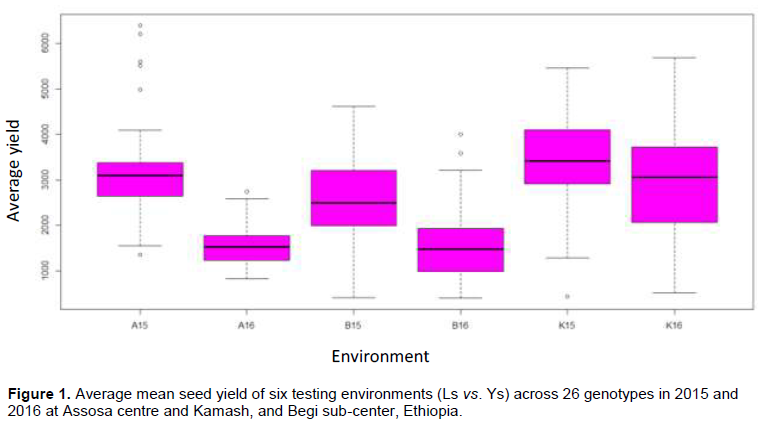
The ANOVA showed that environments have significantly (p£0.001) affected the seed yield of 26 tested genotypes (Table 2). The mean was highly varying with a range of 1545.79 at B16 to 3396.61 kg/ha at K15 for L vs. Y wise combined data analysis (Figure 1). The higher mean at Kamash might be due to soil fertility variation indicating that Kamash is a more potential site for soybean production (Table 1). The mean was reduced by 47.6% at Begi due to location effect (Figure 1). The genotypes produced low yield at areas where soil fertility is a limiting factor as compared to those grown at a fertile soil. The soil at Kamash is more favorable for plant growth than Assosa and Begi with N (0.22 vs. 0.18 and 0.17%), P (18.8 vs. 4.3 and 14.8), K (1.73 vs. 0.17 and 1.5%), and pH (6.51 vs. 5.48 and 5.94), respectively (Table 1). The results of combined ANOVA also showed significant (p£0.001) differences for genotypes (Table 2). This significant genotypes variance indicates adequate genetic variability. Strongly significant (p£0.001) G, E, and GEI variances were reported by Fayeun et al. (2016). The G5 (3202.2), G19 (3170.9), and G17 (2933.2 kg/ha) were proved for the highest mean, ranked 1st, 2nd, and 3rd, respectively. The G5 and G19 were significantly superior except G17, G4, G13, G25, G3, and G6 (Table 5). Seven genotypes (G8, G9, G10, G11, G14, G15, and G16) were low yielding. The G3, G4, G12, G13, and G23 showed specific adaptability only at favorable sites (Figure 2). The GEI MS was also strongly significant (p£0.001) and it might result from magnitude differences changing among tested genotypes (Table 4). This GEI effect was approved by the 1st and 2nd axes consisting both positive and negative values that resulted in cross-over-type interaction (Table 5). Strongly significant GEI effect was also reported by Fekadu et al. (2009). The breeders should be looking either for non-cross-over or absences of GEI effect in selecting of broadly adapting genotypes (Matus Cadiz et al., 2003).
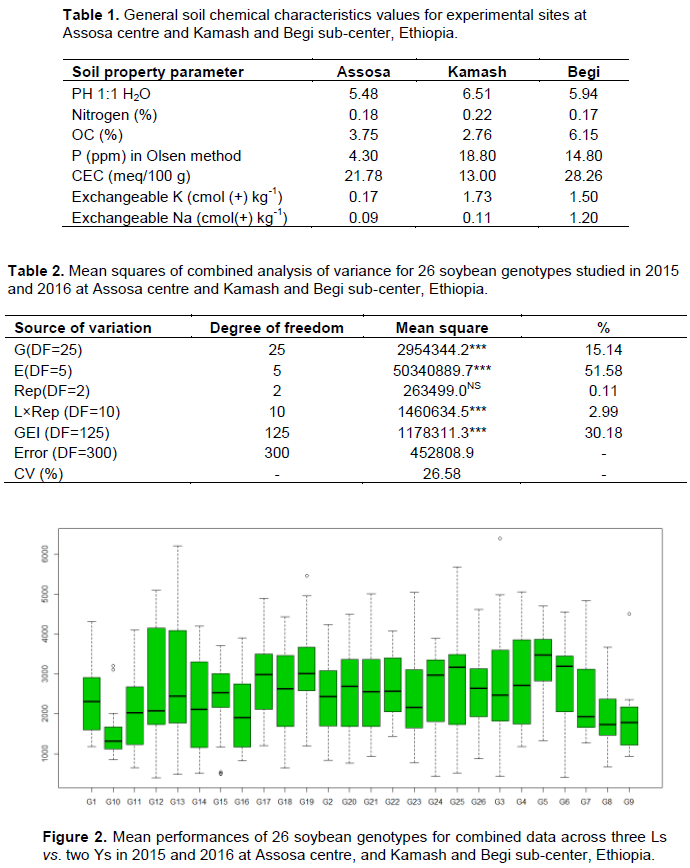
The TTSS of ANOVA due to G+E+GEI was partitioned into G, L, Y, GLI, GYI, LYI, and GLYI variances attributed 15.1, 20.9, 25.5, 15.9, 5.5, 5.2, and 8.8%, respectively (Table 3). The largest variance was explained by E (51.6%) consisted L, Y, and LYI effects. The GEI variance was also almost twice than the G that explained 30.2% of G+E+GEI variance. The interaction is not ignored for such large GEI than G (Yan and Kang, 2002). This large GEI effect was suggested by the differential responses of genotypes and possibility of ME existence with different winning genotypes (Yan and Kang, 2003; Fayeun et al., 2016). The larger GEI variance also indicated both predictable and unpredictable effects leading to specifically or broadly performing genotypes developing (Dehghani et al., 2006).
The ANOVA due to G+L+GLI also provided G, L, and GLI variances (Table 4). The G and GLI variances were 28.3 and 50.3%, respectively, out of the 94.4% for 2015. The G and L effects were also 27.1 and 50.1%, respectively, from total 96.9% variance for 2016. The GLI variance in comparison with G effect suggested the possibility of ME existence. This large variation due to G, L, and GLI effects suggested the suitability of SREG model for stability analysis (Gauch and Zobel, 1996). The GGE model is efficient for G vs. cross-over-type GEI effect interpretation (Karimizadeh et al., 2013). This model is also effective to identify highly stable vs. specifically adapting genotypes via GEI variance demonstrating vs. ME's delineating (Santos et al., 2016). Moreover, Kang et al. (2006) confirmed that the GGE biplot strength for stability vs. superiority was determined. The limitation of GGE biplot is the capturing of small portion of total variability (Yang et al., 2009).
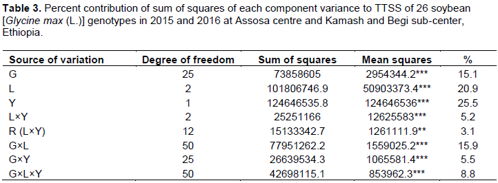
The ANOVA of site regression model was significant (p<0.001) for G, E, and GEI variances (Table 6). The E (53.23%) and GEI (31.15%) effects took the largest proportion of the TTSS variance. The GGE MS variance was strongly significant for PC1, PC2, and PC3 with 81 df, cumulatively accounted 81.95% of the TSS. The 1st and 2nd PC axes with 40.35 and 26.38%, respectively and df of 29 and 27, respectively, effectively partitioned the existed GEI (Table 6). This 66.73% attributes was predicted on the 1st and 2nd PC axes of the total G+GEI derived by G+GE centered to SVD for existed GEI variance visualizing. The results are in accordance with that of Edmore et al. (2015) who explained 36.8% (PC1) and 29.5% (PC2) of the GGE SS. This justifies the efficiency of GGE model in exploiting the G plus GEI variability. Similar reports were confirmed by Yan et al. (2000); Gauch (2013) captured 67% variation with the first two PCs. The positioning of G vs. GEI effects on PC1 vs. PC2 of GGE biplot is as shown in Figure 3. The GGE biplot is an effective method for which-won-where pattern and superiorly performing stable genotypes displaying via
GEI vs. ME's visualizing (Yan et al., 2007; Atnaf et al., 2013; Massaine et al., 2018). The results of GGE biplot showed that G3, G5, G4, G12, G9, and G10 were the highest and poorest located at the vertexes of polygon responding either positively or negatively for seed yield (Figure 3). G3 and G5 were the best winning at A15, B15 and B16, G5 and G4 are the highest, so niche at A16 and K16, while G4 and G12 are also well performing at K15 (Figure 3). The G3 and G12 were specifically adapted at favorable sites; contributed maximum MS to GEI SS due to high values for 2st PC (Figure 3). The polygon vertices are markers for highly projected genotypes indicating specific adaptability (Melkamu et al., 2015; Pavel et al., 2015). G8, G9, G10, G14, and G16 were the poorest that lied in opposite side of the vectors of all environments; not performed at all testing sites. The polygon vertexes G9 and G10 are the poorest genotypes that lied in opposite side of all vectors. Similar results were reported by Ashraful et al. (2017). Moreover, Figure 3 also provides a summary of E vs. G relationship. These variables were represented by vectors and markers, respectively. The correlation between vectors was determined by drawing a lines passed across origin aligned perpendicular to each polygon's sides. The line segments divided the polygon into sites and genotypes sectors. The environments were categorized into three major growing sectors based on the angles related with correlation coefficient (Figure 3). The first group was A15 and B15 with G3 and G5 as the most favorable genotypes. The second sector also includes B16, A16 and K16 where B16 is with G3 and G5, while A16 and K16 are with G5 and G4. The third one is K15 with G4 and G12 as favorable genotypes. The correlation for adjacent vectors was determined by cosine of the angles (Yan and Tinker, 2006). A15 and K15 were higher than 90° projected highly to positive and negative coordinates, respectively, witnessed negative association (Figures 3 and 7). A16, B16, and K16 showed less than 90 which implied strong correlation. This less than 90° indicates high correlation (Yan and Holland, 2010). The positive and negative relations were observed for Ls vs. ys combination analysis (Santos et al., 2016).

The horizontal axis drawn to pass via biplot origin and average genotypes was average tester coordinate (ATC) line used for visual displaying of both means vs. stability (Figure 4). The oval sign of an arrow is showing the positive end of ATC line. The average yielding capacity was estimated by mean projection onto ATC x-axis (Pavel et al., 2015; Ashraful et al., 2017). The double arrowed ATC lines passed via biplot midpoint divided the genotypes into the poorest (below average) vs. the highest (above average), and stable vs. unstable based on means and stability (Figure 4). The G5 is the highest, while G10 is the lowest for mean. The double arrowed ATC lines show the lowest vs. highest and stable vs. unstable genotypes (Fayeun et al., 2016). The stability was also explored by projection onto ATC vertical axis. For instance, G4, G12, G13, G23, G3, and G14 were strongly deviated from ATC line. These genotypes were unstable contributed high MS for GEI effect. The smaller distance between ATC line and genotypes markers also indicates high stability (Figure 4). For example, G5, G17, G25, G26, G15, G7, G16, and G8 were consistent for yield response showing slightly little projection. These shorter absolute deviations witnessed high stability (Melkamu et al., 2015; Fayeun et al., 2016; Ashraful et al., 2017). The term high stability is desirable only when associated with high means (Yan and Tinker, 2006). Moreover, the yield performance consists of both means and stability. Accordingly, the highest scores for PC1 (3.03, 2.25, 3.93, and 2.36%) and near zero absolute values for PC2 (0.77, -0.02, -0.93, and 0.13%) were recorded for G5, G17, G19, and G25, respectively (Table 1). The GGE biplot is effective to evaluate and rank the genotypes based on the means vs. stability (Yan et al., 2007; Amira et al., 2013; Pavel et al., 2015). The GGE biplot was also used to integrate both superior means vs. stability (Kang, 2002; Kang and Magari, 1996). According to Yan (2001), Yan and Hunt (2001, 2002) and Yan and Kang (2003), the first two PCs of GGE biplot are completely partitioning the GEI by visual displaying of G vs. GEI effects distribution, both poor vs. superior, and which-win-where vs. stability pattern for identifying and integrating of superior vs. stability as well as discriminating vs. representing ME mapping.
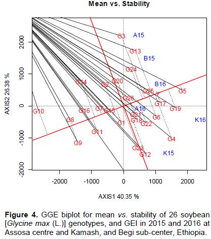
The ATC line drawn to pass via average genotypes vs. biplot origin serves as reference to compare the genotypes based on means and stability. This ATC performance line was used for genotypes ranking according to the mean and stability (Yan and Kang, 2003). The average means for genotypes were estimated by projection onto ATC horizontal axis (Figure 5). The projection is equal to the longest vectors of all genotypes. The center of concentric circles is showing the virtual ideal genotypes (Figure 2). The ideal genotypes could be high yielding and absolutely better for stability (Yan and Kang, 2003; Pavel et al., 2015). The smaller distance from ideal genotype indicates absolute stability. The highest yielding G5 following G19, G17, and G25 was high for both means and stability. The closely positioned genotypes were highly desirable due to high means and stability (Pavel et al., 2015; Richmond et al., 2015; Fayeun et al., 2016). The genotypes located near to ideal genotype were also highly productive and stable (Olayiwola et al., 2015; Ashraful et al., 2017; Massaine et al., 2018). The G10, G8, and G9 were highly projected from the center of concentric circles to unstable. Moreover, the G13 and G18 are not different from apparently inferior G20 and G1 (Figure 5). These highly projected genotypes were found to be the poorest and unstable (Edmore et al., 2015; Massaine et al., 2018). There were different genotypic groups observed from overall inter-relationship among all 26 tested genotypes (Figures 5 and 7). The G17, G19, and G25 were found to be positively and moderately correlated with most favorable G5 (Figure 5). There are high correlation among the best genotypes namely G5, G17, G19, and G25 (Figure 5). The G6, G19, G25, G26, and G21 had shown positively strong association with the most favorable genotypes (G17 and G5) (Figure 7). Similar results of strong correlation among the genotypes were reported by Ashraful et al. (2017). They confirmed that the genotypes being positioned close to each other on GGE biplot responding together similarly to the environments were found near to these genotypes.

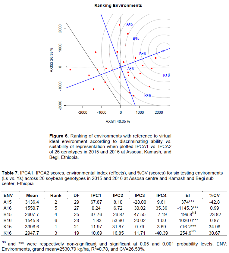
The average environment coordination (AEC) line was passed via average environment vs. origin for ideal environment position delineation. The average means was estimated by projection onto AEC horizontal axis. The projection is equal to the longest vectors of all environments. The center of concentric circles shows virtual ideal environments. The deviation is zero indicating absolutely representative for average environments. The representing vs. discriminating ability was also explored by length of projection (Figure 6). The AEC concentric circle GGE biplot method is best to estimate the discriminating vs. representing ability for assessing the genotypes (Yan and Tinker, 2006; Yan et al., 2007; Atnaf et al., 2013). For instance, the suitability of B16 and K16 were high in representing all genotypes. The concentric circles nearest sites were high for their stability in representing the genotypes (Fayeun et al., 2016; Ashraful et al., 2017). The discriminating ability was significant and positive for A15 and K15 where they deviated strongly from the center of the concentric circles (Table 7 and Figure 6). The closer it is the better it will be as virtual ideal environment to all tested soybean genotypes. The K16 is highly favorable in representing all the tested genotypes considering both mean vs. stability. The ideal environments are close to ATC x-axis and zero projection onto ATC y-axis (Ashraful et al., 2017). Moreover, Blanche and Myers (2006) also witnessed the efficiency of GGE for ideal genotypes vs. highly representing optimum environment identification for widely adapted genotypes selection.
The yield data vs. PC coordinates plotting for additive and interaction effects was done on the same biplot for yield variation efficiently partitioning. The A16 and B16 exhibited nearly additive effect on genotypes (Figure 7). The yield performance at A16 and B16 was associated with overall mean confirmed average responses to genotypes. The strongly projected sites were highly discriminated to all genotypes. The A15 and K15 were the longest which showed high yield variation for genotypes. The genotypes consistencies were better at A16 and B16 than inconsistent responses at A15 and K15 (Figure7). Environments with longer vectors are high in discrimination capability to all tested genotypes (Yan et al., 2007; Massaine et al., 2018). The results of the present study were strongly allied with Fayeun et al. (2016) who noticed little variation to genotypes for short vectors, while high variation for strongly projected testing sites. Similarly, the entries positioned near to the biplot origin were taken as an average means (Figure 7). For instance, G1, G18, G15, G21, and G26 showed average response for their yield means. G4, G5, G12, and G13 were the highest for their means being strongly projected from the center of the biplot. G3, G8, G9, and G10 were the poorest genotypes being deviated negatively (Figure 7). These polygon vertexes positively vs. negatively responding genotypes were unstable, adapted specifically at favorable environments (Melkamu et al., 2015). These two variables projection showed that the GEI which resulted from regressing of G over E as well as E over G contributed high MS for GEI variance. This resulted in inconsistency of the genotypes for mean performance due to strongly significant GEI effect in MEVT.
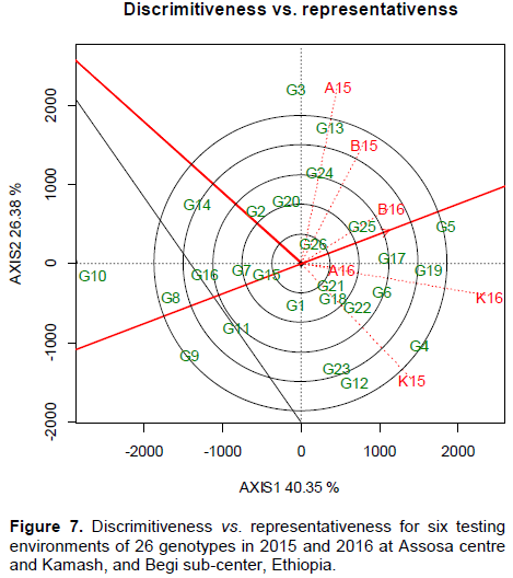
The angles present between the average tester axes vs. biplot vectors indicated the environmental stability (Figure 7). The distance between the biplot vectors represented the similarity vs. differences in discriminating vs. representing to all tested genotypes (Fayeun et al., 2016). The environments near to AEC are high for their stability. Accordingly, K16, B16, and A16 were less than 90° that deviated little from AET axes (Figure7). These averagely responding environments were suitable for widely adapted soybean genotypes selection. Smaller angles for vectors showed strongly positive correlation (Massaine et al., 2018). The results of the present study were also in accordance with Marcin and Krzysztof (2016). A15 and K15 were highly projected from AET showing high discriminating ability to all genotypes. Similar results were reported by Fayeun et al. (2016) and Bhartiya et al. (2017).
CONCLUSION
The pooled ANOVA showed strongly significant G, E, and GEI variances with CV of 26.58%, mean of 2530.79 kg/ha, and R2 of 0.78%. The TTSS was partitioned into G, E, and GEI for MS contribution. The maximum was contributed by E (51.6%) followed by GEI (30.2%). The main variability is therefore due to the E and GEI. Genotypes G3, G5, G4, G12, G9, and G10 were located at corners of the polygon. Genotypes G3 and G12 were unstable significantly contributing to GEI due to high scores for PC2. Genotypes G5, G17, G19, and G25 were high for PC1 and near zero for PC2. This indicated high stability and heritability growing vigorously in producing maximum means might be due to broad sense genetic constituent for yield vs. stability so there are high selection probability and possibility for wide adaptability. These consistently performing ideal genotypes were proved for yield contributing desirable characters. Therefore, including these lines in future breeding programs would be advised in enhancing soybean productivity in Ethiopia. These two seasons vs. three locations data were used for GGE stability analysis; accordingly, further GGE vs. AMMI models GEI effect partitioning for G vs. L vs. Y should be considered with the objectives of promising (means vs. stability) genotypes exploring for both specific and broad adaptability.
CONFLICT OF INTERESTS
The author has not declared any conflict of interests.
ACKNOWLEDGEMENTS
The author thanks Ethiopian Institute of Agriculture Research for providing funds for the study and appreciates Assosa Center Soil Lab staff for unlimited duties in soil analysis and also Lowland Oils Breeding staff for their genuine help in data measuring.
REFERENCES
|
Amare B (1987). Progress and future prospect in soybean research in Ethiopia. In: Proc 19th National crop improvement Conefrence. Institute of agricultural Research, Addis Ababa, Ethiopia pp. 252-265 |
|
|
Amira JO, Ojo DK, Ariyo OJ, Oduwaye OA, Ayo Vaughan MA (2013). Relative discriminating powers of GGE and AMMI models in tropical soybean genotypes selection. African Crop Science Journal 21(1):67-73. |
|
|
Ashraful A, Farhad, Abdul H, Naresh CDB, Paritosh KM, Mostofa AR, Amir H, Mingju L (2017). AMMI and GGE biplots for wheat genotypes yield stability in Bangladesh. Pakistan Journal of Botany 49(3):1049-1056. |
|
|
Assosa Agricultural Research Center Farming System Survey (AsARCFSS) (2007). Assosa, Ethioipa. |
|
|
Assosa Agricultural Research Center Metrology Station (AsARCMS) (2016). Assosa Research Center Weather Data Base Generation, and Management for Agricultural Research System Information Accessing. Assosa, Ethioipa. |
|
|
Atnaf M, Kidane S, Abadi S, Fisha Z (2013). GGE biplots to analyze soybean MET data in north Western Ethiopia. Journal of Plant Breeding and Crop Science 5(12):245-254. |
|
|
Bhartiya A, Aditya JP, Kamendra S, Pushpendra P, Purwar JP, Anjuli A (2017). AMMI, and GGE analysis of MET of soybean in North Western Himalayan state Uttarakhand of India. Legume Research: An International Journal 40 (2):306-312. |
|
|
Blanche SB, Myers GO (2006). Identifying discriminating location selection in Louisiana. Crop Science 46: 946-949. |
|
|
Burgueno J, Crossa J, Vargas M (2001). SAS Programs for graphing GE and GGE biplots," CIMMYT, INT. Mexico. |
|
|
Dehghani H, Ebadi A, Yousefi A (2006). Biplot analysis of GEI for barley yield in Iran. Agronomy Journal 98:388-393. |
|
|
Ding M, Tier B, Yan W (2007). GGE Analysis for G, E, and GEI effects on P. Radiata. Paper for AFGCB on Wood Quality, 1114 H.T, Australia. |
|
|
Edmore G, Peter SS, Caleb MS (2015). GGE biplot sorghum genotype evaluation. Canadian Journal of Plant Science 95:1205-1214. |
|
|
Fayeun LS, Alake GC, Akinlolu AO (2016). GGE Biplot analysis of fluted pumpkin (Telfairia occidentalis) landraces evaluated for marketable leaf yield in Southwest Nigeria. Journal of the Saudi Society of Agricultural Sciences. (In Press). Genotype x environment interactions and stability of soybean for grain yield and nutrition quality. African Crop Science Journal 17(2). |
|
|
Gauch HG (2006). Statistical analysis of yield trials by AMMI, and GGE biplots. Crop Science 46:1488-1500. |
|
|
Gauch HG (2013). A simple protocol for AMMI analysis of yield trials. Crop Science 53:1860-1869. |
|
|
Gauch HG, Zobel RW (1996). AMMI Analysis of yield. CRC Press, Boca Raton, FL: pp. 85-122. |
|
|
Hymowitz T (1970). Domestication of the soybean. Economic Botany 24:408-421. |
|
|
Institute of Agricultural Research (1982). Soybean production guideline. Adis Ababa, Ethiopia. |
|
|
Kang MS (1998). Using GEI for crop cultivar development. Advances in Agriculture 62:199-252. |
|
|
Kang MS (2002). GEI effect: Progress, and prospects: In MS Kang (ed.) Quantitative genetics, genomics, and plant breeding. CABI Publ., Wallingford, Oxon, UK. pp. 221-243. |
|
|
Kang MS, Aggarwal VD, Chirwa RM (2006). Adaptability, and stability of bean cultivars as determined via yield stability statistic, and GGE analysis. Journal of Crop Improvement 15:97-120. |
|
|
Kang MS, Magari R (1995). Program for calculating stability, and yield stability statistic. Agronomy Journal 87:276-277. |
|
|
Kang MS, Magari R (1996). New developments in selecting for phenotypic stability in Crop Breeding. In Kang MS, Gauch HG Jr (ed.) GEI. CRC Press, B.R., FL. p: 1-14. |
|
|
Karimizadeh R, Mohammadi M, Sabaghni N, Mahmoodi AA, Roustami B, Seyyedi F, Akbari F (2013). GGE biplot stability analysis of yield in MET of lentil genotypes. Notulae Scientia Biologicae 5:256-262. |
|
|
Kaya Y, Aksura M, Taner S (2006). GGE-biplot analysis of multi-environment yield trials in bread wheat. Turkish Journal of Agriculture and Forestry 30(5):325-337. |
|
|
Lackey JA (1977). A Synopsis of Phaseoleae (Leguminosae): Ph.D. Dissertation. Iowa University. America, Iowa. |
|
|
Marcin K, Krzysztof U (2016). Application of GGE biplot in MET on selection of forest trees. Folia Forestalia Polonica, Series A Forestry 58(4):228-239. |
|
|
Massaine BES, Kaesel JDS, Maurisrael DMR, Jose ANDMJ, Laize RLL (2018). GEI effect analysis in cowpea lines by GGE Biplot. Revista Caatinga 31(1):64-71. |
|
|
Matus Cadiz MA, Hucl P, Perron CE, Tyler RT (2003). GEI for grain color in wheat. Crop Science 43:219-226. |
|
|
Melkamu T, Sentayehu A, Firdissa E (2015). GGE Biplot GEI, and yield stability analysis of bread wheat genotypes in South East Ethiopia. World Journal of Agricultural Sciences 11(4):183-190. |
|
|
Olayiwola MO, Soremi PAS, Okeleye KA (2015). Evaluation of some cowpea [Vigna unguiculata (L.) Walp.] genotypes for stability of performance over 4 years. Current Research in Agricultural Sciences 2(1):22-30. |
|
|
Pavel S, Nataliya V, Aleksey N, Olga S, Olga V, Olga B, Yuriy L (2015). GGE biplot analysis of GEI of spring barley varieties. Zemdirbyste Agriculture 102(4):431-436. |
|
|
Rao MS, Mullinix BG, Rangappa M, Cebert E, Bhagsari AS, Dadson RB (2002). GEI effect and soybean varieties stability analysis. Agronomy Journal 94:72-80. |
|
|
Richmond EE, Godson E, Lawrence SF (2015). AMMI vs. GGE models soy yield assessment in many environments in Humidorest Fringes of Southeast Nigeria. Agricultura Tropica et Subtropica, 48(3-4):82-90. |
|
|
R-Software V-3.4.3 (2017). R-Foundation for Statistical Computing Platform: x86_64-w64-mingw32/x64 (64-bit). |
|
|
Santos A dos, Ceccon G, Teodoro PE, Correa AM, Alvarez R de CE, Figueiredo da Silva J, Alves V (2016). Adaptability vs. stability of cowpea genotypes via REML/BLUP vs. GGE biplot. Bragantia, 75(3):299-306. |
|
|
Statistical Analysis System (SAS) (2002). SAS/STAT 9 User Guide. SAS Institute, Cary, NC, USA. |
|
|
Summerfied RJ (1975). Effects of day length, and night temperatures on soybean: Physics Work shop, IITA. |
|
|
Yan W (2001). GGE biplot: Window application for graphical analysis of ME two way data. Agronomy Journal 93:1111-1118. |
|
|
Yan W (2014). Crop variety trial: data management, and analysis, Wiley-Blackwell 360 p. |
|
|
Yan W, Holland JB (2010). A heritability adjusted GGE biplot for test environment evaluation. Euphytica 171:355-369 |
|
|
Yan W, Hunt LA (2001). Interpretation of GEI for winter wheat yield in Ontario. Crop Science 41:19-25. |
|
|
Yan W, Hunt LA (2002). Biplot analysis of diallel data. Crop Science 42:21-30. |
|
|
Yan W, Hunt LA, Sheng Q, Szlavnics Z (2000). GGE Biplot Variety Testing, and MEI. Crop Science 40:596-605. |
|
|
Yan W, Kang MS (2002). GGE biplot analysis: A graphical tool for breeders, geneticists, and agronomists. CRC press. |
|
|
Yan W, Kang MS (2003). GGE Biplot Analysis: A Graphical Tool for Breeders, Geneticists, and Agronomists. CRC Press, Boca Raton, Florida. |
|
|
Yan W, Kang MS, Ma B, Woods S, Cornelius PL (2007). GGE vs. AMMI biplots analysis of GEI data. Crop Science 47:643-655 |
|
|
Yan W, Tinker NA (2006). Biplot analysis of MET data: principle, and application. Canadian Journal of Plant Science 86:623-645. |
|
|
Yang R, Crossa J, Cornelius PL, Burgueno J (2009). Biplot analysis of GEI effect. Crop Science 49:1564-1576. |
|
|
Zobel RW, Wright MJ, Gauch HG (1988). Statistical analysis of a yield trial. Agronomy Journal 80:388-393. |
|
Copyright © 2024 Author(s) retain the copyright of this article.
This article is published under the terms of the Creative Commons Attribution License 4.0


