ABSTRACT
Lake Malawi continues experiencing serious depletion of most valuable fish species. Presently, commercial and artisanal fishery are forced to target less valuable fish species. Evidently, economic importance of Engraulicypris sardella in Malawi cannot be negated as it currently contributes over 70% of the total annual landings. However, such highest contribution could be a sign of harvesting pressure. Therefore, as the species continues being increasingly exploited, the development of scientific understanding through application of stochastic models is particularly relevant for present and future policy making and formulation of strategies to sustain the resource in the lake. Thus, the study was designed to forecast the annual catch trend of E. sardella from Lake Malawi. The study used time series data from 1976 to 2015 period obtained from Monkey Bay Fisheries Research Station of the Malawi Fisheries Department. The study adopted Box-Jenkins procedures to identify appropriate Autoregressive Integrated Moving Average (ARIMA) model, estimate parameters in ARIMA model and conducting diagnostic check. The study findings showed that ARIMA (2,1,1) model had least Normalized Bayesian Information Criterion (NBIC) value making it a appropriate model for the study. ARIMA (2,1,1) model showed that E. sardella annual catches are positively fluctuating. Again, the model predicted that E. sardella annual catches from Lake Malawi will increase from the annual total landings of 71,778.47 metric tons to 104,261.20 metric tons in the next 10 years (ceteris paribus).
Key words: Box-Jenkins, Engraulicypris sardella, Lake Malawi, autoregressive integrated moving average (ARIMA), Modelling, Usipa, Stochastic.
Engraulicypris sardella locally known as Usipa is one of the endemic fish species in Lake Malawi. The species belongs to the Cyprinid family. Literature suggests that the biology of E. sardella is very contentious. In early 1960s, Iles (1960) noted that the life cycle of E. sardella can normally be completed within 1 year. However, Morioka and Kaunda, (2004) argued that the species has an extended breeding periods. Morioka and Kaunda, (2004) further claimed that the fact that the species has an extended breeding periods is a strong evidence of the existence of plural stocks meaning that different stocks of E. sardella may adapt to the different optimum temperature for reproduction. However, because fisheries scientists, ecologists and managers have not yet found a substantial evidence on this contentious biology and life span of E. sardella, it has been difficult to set management recommendations and strategies to sustain E. sardella stocks in Lake Malawi. Similar observation was made by Allison et al (1996). Unfortunately, the economic importance of Engraulicypris sardella in Malawi cannot be negated as it currently contributes over 70% of the total annual landings (Department of Fisheries, 2017).
Furthermore, it has been noted that fish catches in the past two years have shown a positive catch fluctuation with estimated annual catch of 30,000 metric tonnes to 80,000 metric tonnes as of 2010 and a significant catch contribution has been from E. sardella and Haplochromine species (GoM, 2015). On the other hand, it has also been noted that Lake Malawi continues experiencing serious depletion of most valuable fish species. Presently, both commercial and artisanal fishery have been forced to target less valuable fish species such as E. sardella and Haplochromine species (Hara and Njaya, 2016). It is very apparent that the shifting will consequently increase harvesting pressure on the resource. Therefore, as the species continues being increasingly exploited, the development of scientific understanding through application of stochastic models is relevant for present and future policy making and formulation of strategies to sustain the resource in the lake (Cohen and Stone, 1978). Thus, the study was designed to forecast the annual catch trend of Lake Malawi E. sardella using stochastic models.
Data collection
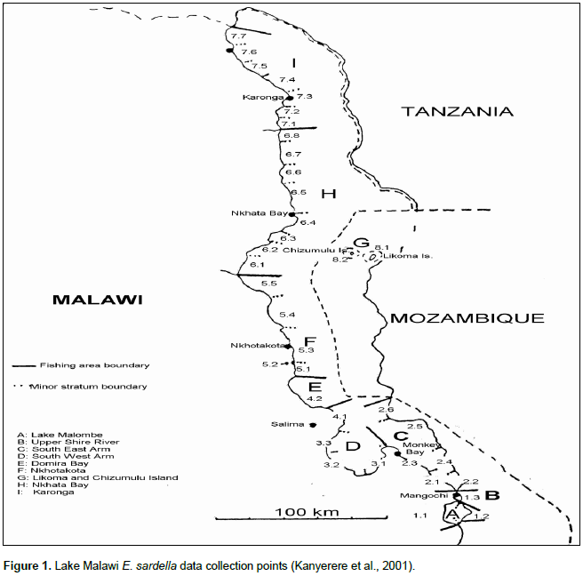
Figure 1 shows E. sardella data collection points. Literature shows that Malawi Department of Fisheries started collecting E. sardella catch data in early 1970s from beach recorders using a random sampling technique introduced by FAO (Bazigos, 1972). However, it was noted that data collected from the beach recorders during 1970s to 1975 were not tested for its statistical realiability (Bazigos, 1972). Because of such suspicions, the study used the time series data of E. sardella total landings from 1976 to 2015 period. The data was obtained from Monkey Bay Fisheries Research Station of the Malawi Fisheries Department. The unit of measurement referred to the weight of fish at the time of removal from water was expressed in metric tons. For the purpose of data collection, Lake Malawi is coded into several sections also known as strata (refer to Figure 1). E. sardella data is collected by employing random selection of a series of landing sites within each established sampling frame taking into consideration the mobility patterns among the fishermen within the fishing community. The actual survey at each sampling site includes all crafts/fishing gears or in the case of larger fishing communities sub-sampling of the crafts/fishing gears. It is very important to note that Mangochi district only uses gear based sampling called Malawi Traditional Fishery (MTF) and the rest of the districts use craft based sampling known as Catch Assessment Survey (CAS). The survey is conducted by the actual weighing of the catch of the selected landings and interviewing the fishermen especially on the effort exerted to produce the landed catch.
Stationarity test
To check whether E. sardella time series data needed to be differenced to make it stationary or not, Dickey-Fuller t-statistics test was carried out. The mathematical model of -Dickey- Fuller test is given below (Dickey and Fuller, 1976):

The Dickey-Fuller t-test was based on the fact that accepting null hypothesis implies that the data needs to be differenced to make it stationary.
Derivative of stochastic models
Autoregressive (AR) model
As suggested by Box and Jenkins, the (AR) which is a component of ARIMA model was mathematically expressed as (Box and Jenkins, 1970):
Moving average (MA) model
The MA model was defined as (Box et al. 2015):
The Autoregressive Moving Average (ARMA) Model
Autoregressive (AR) and Moving Average (MA) models were combined to form ARMA (p, q) model mathematically expressed as (Cochrane, 1997):
The Autoregressive Integrated Moving Average (ARIMA) Model
In ARIMA models, a non stationary data is made stationary by applying log-difference transformation (Minović, 2008) or finite differencing which transforms non stationary time series data into stationary (Stoffer and Dhumway, 2010). The general mathematical expression of ARIMA (p, d, q) model is (Lombardo and Flaherty, 2000):

here p, d and q are integers greater than or equal to zero and refer to the order of the autoregressive, integrated and moving average parts of the model respectively. The integer d controls the level of differencing.
Model Identification
Parameters estimation
The Maximum Likelihood test (ML), least square estimation method and Yule-Walker statistical procedures were used to estimate the parameters and the corresponding standard errors.
Diagnostic checking
Box and Jenkins (1970) developed a practical approach to build ARIMA model, which best fit a given time series and also satisfy the parsimony principle. Generally, this step involved the analysis of the residuals as well as model comparisons (Chang et al., 2012). The Ljung-Box Q was used in the diagnostic test. Mathematically, the Ljung-Box Q was expressed as (Box et al. 2015)
where

is the estimated autocorrelation of the series at lag
k and
m is the number of lags being tested.
The hypothesis of Ljung-Box test was:
H0: Residual is white noise
H1: Residual is not white noise
If the sample value Q exceeds the critical value of X
2 distribution with
m degree of freedom, then at least one value of

is statistically different from zero at the specified level of significance. Again, Bayesian Information Criterion (BIC) was employed to evaluate the adequacy of AR, MA and ARIMA processes. Bayesian Information Criterion (BIC) developed by Gideon Schwarz (Schwarz, 1978) was used to select the model among a finite set of models. BIC model was computed as
Model fitting and Prediction
Upon identification of optimum model and estimating all parameters, the forecast of E. sardella catch landing from 2015 to 2025 was made. All inferential and descriptive statistics were performed using STATA 14 (StataCorp, 2015)

Stationarity test
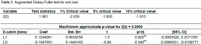
The stationarity test was done by applying Dickey-Fuller statistical test. The test was done to determine whether time series data had a unit root or not (Hamilton, 1994). The results are presented in Table 1. The basic null hypothesis of Dickey-Fuller statistical test was that
E. sardella time series data had a unit root. According to Dickey and Fuller (1976), if unit root is found in a series, it implies that more than one trend is present in the series. As seen from Table 1, the Z-score yielded by the Dickey-Fuller statistical test showed that
E. sardella time series data had a unit root. The Z(t) test statistics fell within the range of acceptance interval
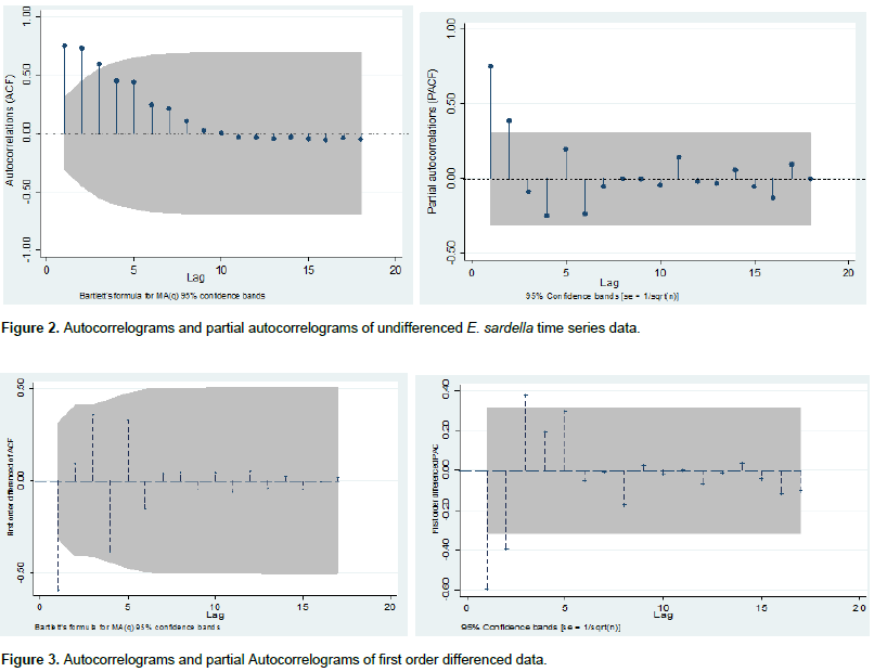
which explained that the data had to be differenced to make it stationary. Furthermore, Figure 2 shows that the mean of the series appears to be non-stationary with an average return not equal to zero. To transform the data from non stationary to stationary, first order differencing of the data was conducted using natural logarithms (Box et al. 1978). The results are presented in Figure 3. Enders (2004) noted that the first-differencing of the time series data mitigates the effects of the trend and controls seasonarity. Figure 2, shows that the mean of the series were stationary with an average return of approximately zero. The autoregressive model of order p(AR (q)) was stationary and moving average model of order q(MA (q)) was perfect.
Model Identification
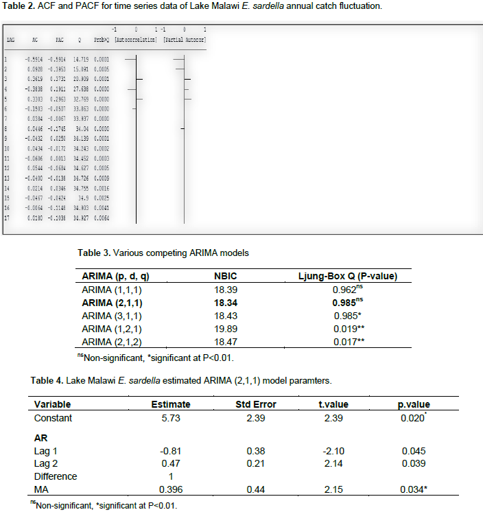
As seen from Figure 2, the autocorrelation and partial autocorrelation coefficients (ACF and PACF) were ploted and the type and order of the adequate model required to fit the series was determined. Table 2 shows the autocorrelation and partial autocorrelation coefficients (ACF and PACF) of various orders of differenced series of data. The coefficients presented in Table 2 were used to identify various ARIMA models together with their corresponding fit statistics. Table 3 shows the results of various competing ARIMA models. It was very interesting to note that ARIMA (2,1,1) model in Table 3 was the best model among all other competing models. Table 4 shows the estimated values of the ARIMA (2,1,1) model. The Ljung-Box Statistic test of ARIMA (2,1,1) model was not signficantly (p>0.05) different from zero. The P. value was significantly higher (0.985) comparing to the critical value (0.05). This implied that the null hypothesis of white noise, had to be rejected. Rejecting the null hypothesis of white noise implied that the ARIMA (2,1,1) model was capable of adquately capturing the correlation in the time series. According to Czerwinski et al (2007), the residuals were independently distributed in the population from which sample size was taken. It was further noted that the coefficients of parameters of ARIMA (2,1,1) model were all significant (p<0.05) and had least Normalised BIC value. Czerwinski et al (2007) suggested that the best ARIMA model with accurate forecasts must have lowest Normalised BIC and model parameters must be significant (p<0.05). This presents a substantial justification why the ARIMA (2,1,1) model was mostly prefered in the study.
Model Diagnostic Check
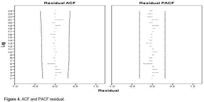
The ARIMA (2,1,1) model was further subjected to autocorrelations and partial autocorrelations of residuals of various orders. Figure 4 shows the various autocorrelations of up to 24 lags. From the plots of the residual ACF and PACF, it was very apparent that, the ARIMA (2,1,1) model was confirmed to be adequate in the sense that the points below and above were all uneven suggesting that the model was fit. Also, the individual residual autocorrelations were very small and generally within 95% level of confidence suggesting that the selected model was fit.
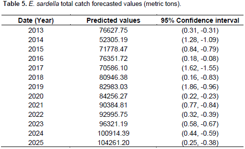
Forecasting
The ARIMA (2,1,1) model forecasted E. sardella total landings from 1976 to 2025. For the preciseness and accurateness sake, observations only from 2013 to 2025 have been presented in Table 5. Figure 5 shows the forecasted value from 1976 to 2025. Figure 5 further shows that E. sardella total landing is fluctuating with positive trend as it decreases and increases at some point. The model (2,1,1) in Figure 5 further predicted that there is high probability that E.sardella catches from Lake Malawi will increase up to 104261.20 metric tons by 2025. The positive annual catch trend depicted by the model could be a sign of harvesting pressure exerted upon the species by the fishers. Figure 6 shows that there has been stability in total annual landings from 1993 to 2004. The lowest E. sardella total annual landing was recorded in the year 1993 and the highest in the year 2015. Generally, E. sardella total annual landings fluctuation has been showing positive trend from 2004 to 2015 with some troughs in 2011 and 2012 and then another drop two years later. It has been noted that low efficiency to harvest the field was reported from 1993 and lasted for11 years. As observed by Hara and Njaya (2016), the positive trend of E.sardella total landings among other reasons could be attributed to the fact that many fishers are currently targeting usipa much more than utaka because of the far much better catches of the former compared to the latter for similar effort.
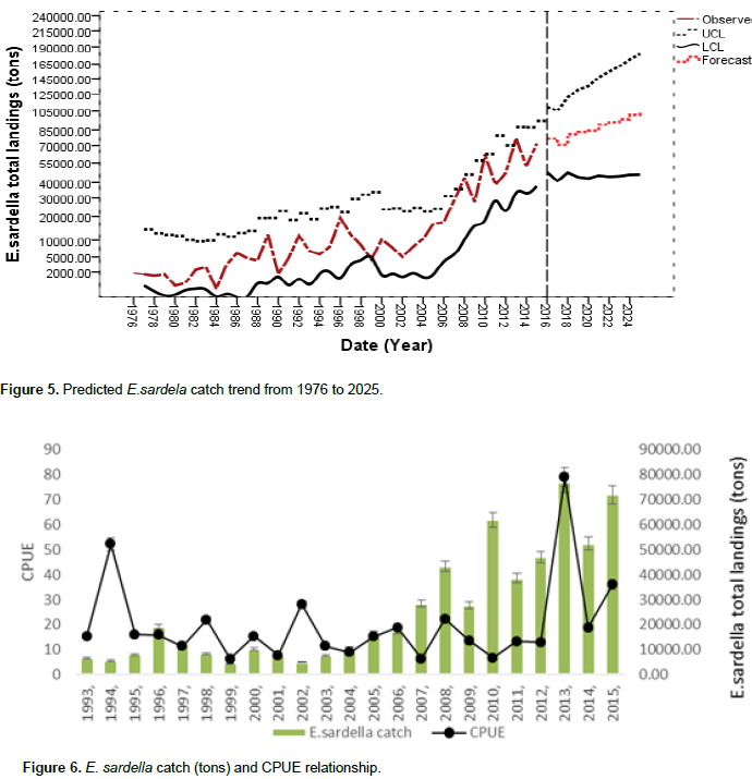
In fisheries and conservation biology, the catch per unit effort is an indirect measure of how abundant a targeted species is (Puertas and Bodmer, 2004). In other words, the fishing efficiency which is known as catch per unit effort (CPUE) is an index of abundance which to some extent provide relevant information on how much fish is in the water. As seen from Figure 6, the CPUE of E. sardella has been fluctuating throughout. Such fluctuation indicates that E.sardella population diversity is unstable. As seen from Figure 5, CPUE fluctuated positively from 1993 to 1994 and from 1994 to 1995, the CPUE trend decreased rapidly and since then, there has been a slight fluctuation up to 2012 despite increasing in E. sardella catches from 2007 to 2012. From 2012 to 2013, the CPUE trend increased and recorded highest in 2013 and also corresponded to the highest E.sardella total landings. The general increasing trend of CPUE in 2013 indicated that E. sardella fishery was in good health and the fishery was yet to reach its maximum sustainable yield (MSY). From 2013 to 2014, the CPUE decreased sharply while E.sardella catch trend remained high. According to Puertas and Bodmer, (2004), deceasing in CPUE indicated overexploitation while increasing CPUE indicated underexploitation. However, if the CPUE were to register stable, then it could indicate sustainable harvesting. Since CPUE is unstable, it means that E.sardella fishery requires proper management plans because human population will obviously surpus (Malthus, 1798) the capacity at which E. sardella can reproduce and when that happens, such positive trend may likely collapse in the near future especially in the years of low recruitment.
The study findings showed that ARIMA (2,1,1) model had least Normalized Bayesian Information Criterion (NBIC) value making it a appropriate model for the study. ARIMA (2,1,1) model showed that E. sardella annual catches are positively fluctuating. Again, the model predicted that E. sardella annual catches from Lake Malawi will increase from the annual average level of 71,778.47 metric tons to an average of 104,261.20 metric tons in the next 10 years (ceteris paribus). However, regardless of the model projecting future positive fluctuation of E. sardella total landings, the catch per unit effort (CPUE) has been fluctuating throughout. Such fluctuation indicates that E.sardella population diversity is unstable and requires proper management plans because human population will obviously surpass the capacity at which E. sardella can reproduce and when that happens, such positive trend will likely collapse in the near future especially in the years of low recruitment.
Despite the fact that the ARIMA (2,1,1) model predicted that E. sardella total landings will increase for the next 10 years, the CPUE shows to be unstable, which means that E. sardella fishery requires proper management plans to ensure its sustainability.
The authors have not declared any conflict of interests.
The authors wish to extend gratitude to Momkey Bay Research Station of the Department of Fisheries for providing E.sardella catch data for the sudy.
REFERENCES
|
Allison E, Irvine K, Thompson A, Ngatunga B (1996). Diets and food consumption rates of pelagic fish in Lake Malawi, Africa. Freshwater Biol. 35:489-515.
Crossref
|
|
|
|
Bazigos GP (1972). The improvement of the Malawian fisheries Statistical system. A report to the Integrated Project. FAO /MLW /16. Zomba, Malawi.
|
|
|
|
Box G, Jenkins G (1970). Time Series Analysis, Forecasting and Control. San Francisco: Holden-Day.
View
|
|
|
|
Box G, Hunter W, Hunter J (1978). Statistics for Experimenters: An Introduction to Design, Data Analysis and Model Building. Hoboken, NJ, USA: John Wiley and Sons:
|
|
|
|
Box G, Jenkins G, Reinsel G, Ljung G (2015). Time series analysis: Forecasting and Control. Hoboken, NJ, USA: John Wiley & Sons.
|
|
|
|
Chang X, Gao M, Wang Y, Hou X (2012). Seasonal autoregressive integrated moving average model for precipitation time series. J. Math. Stat. 4(8):500-502.
Crossref
|
|
|
|
Clement E (2014). Using Normalized Bayesian Information Criterion (Bic) to Improve Box - Jenkins Model Building. Am. J. Math. Stat. 4(5):214-221:
View
|
|
|
|
Cochrane H (1997). Time Series for Macroeconomics and Finance. Chicago: Graduate School of Business, University of Chicago,Spring.
|
|
|
|
Cohen Y, Stone J (1978). Multivariate time series analysis of the Canadian fisheries system in Lake Superior. . Can. J. Fish. Aquat. Sci. 44 (Suppl. 2):171-181.
Crossref
|
|
|
|
Czerwinski I, Guti’errez-Estrada J, Hernando-Casal J (2007). Short-term forecasting of halibut CPUE: Linear and non-linear univariate approaches. Fish. Res. 86:120-128.
Crossref
|
|
|
|
Department of Fisheries. (2017). Annual Economic Report 2017 Fisheries Sector Contribution. Lilongwe, Malawi: Department of Fisheries.
|
|
|
|
Dickey D, Fuller W (1976). Distribution of the estimators for autoregressive time series with a unit root. J. Am. Stat. Assoc. 74(366):427-31.
Crossref
|
|
|
|
Enders W (2004). Applied Econometric Time Series. 2nd ed. New York: Wiley.
|
|
|
|
GoM (2015). National Biodiversity Strategy and Action Plan II (2015 –2025). Lilongwe: Environmental Affairs Department.
|
|
|
|
Hamilton J (1994). Time Series Analysis. Princeton: Princeton University Press.
|
|
|
|
Hara M, Njaya F (2016). Between a rock and a hard place: the need for and challenges to implementation of Rights Based Fisheries Management in small-scale fisheries of Southern Lake Malawi. Fish. Res. 174:10-18.
Crossref
|
|
|
|
Iles T (1960). Engraulicypris sardella. Joint Fisheries Research Organisation Annual Report, No. 9,. Lusaka: Government Printer.
|
|
|
|
Kanyerere G, Namoto W, Mponda O (2001). Analysis of Catch and Effort Data for the Fisheries of Nkhata Bay, Lake Malawi, 1976-1999. Lilongwe: Fisheries Bulletin No. 48:Department of Fisheries.
|
|
|
|
Lombardo R, Flaherty J (2000). Modelling Private New Housing Starts In Australia. Pacific-Rim Real Estate Society Conference (pp. 24-27). Sydney: University of Technology Sydney (UTS).
|
|
|
|
Malthus T (1798). An essay on the principle of poAn essay on the principle of population. Londom: Murray.
View
|
|
|
|
Minović J (2008). Application and Diagnostic Checking of Univariate and Multivariate GARCH Models in Serbian Financial Market. Econ. Analysis 40(1-2):73-87.
|
|
|
|
Morioka S, Kaunda E (2004). Preliminary examination of the growth of mpasa,Opsaridium microlepis (Günther, 1864) (Teleostomi: Cyprinidae), younger than one year old,collected from Lake Malawi. Afr. Zool. 39(1):13-18.
|
|
|
|
Puertas P, Bodmer R (2004). Hunting effort as a tool for community-based wildlife management in Amazonia. In K. Silvius, R. Bodmer, & J. Fragoso., People in Nature: Wildlife Conservation in South and Central America. Columbia: Columbia University Press. pp. 123-136.
Crossref
|
|
|
|
Schwarz G (1978). Estimating the dimension of a Model. Ann. Stat. 6(2):461-464.
Crossref
|
|
|
|
StataCorp (2015). Stata sStatistical Software: Release14. College Station. TX StataCorp LP.
|
|
|
|
Stoffer D, Dhumway R (2010). Time Series Analysis and its Application 3rd Edn. New Yolk: Springer.
View
|


 is the estimated autocorrelation of the series at lag k and m is the number of lags being tested.
 is statistically different from zero at the specified level of significance. Again, Bayesian Information Criterion (BIC) was employed to evaluate the adequacy of AR, MA and ARIMA processes. Bayesian Information Criterion (BIC) developed by Gideon Schwarz (Schwarz, 1978) was used to select the model among a finite set of models. BIC model was computed as

 which explained that the data had to be differenced to make it stationary. Furthermore, Figure 2 shows that the mean of the series appears to be non-stationary with an average return not equal to zero. To transform the data from non stationary to stationary, first order differencing of the data was conducted using natural logarithms (Box et al. 1978). The results are presented in Figure 3. Enders (2004) noted that the first-differencing of the time series data mitigates the effects of the trend and controls seasonarity. Figure 2, shows that the mean of the series were stationary with an average return of approximately zero. The autoregressive model of order p(AR (q)) was stationary and moving average model of order q(MA (q)) was perfect.


